Fitting the Highly Adaptive Lasso with
hal9001
Nima Hejazi, Jeremy Coyle, Rachael Phillips, Lars van der Laan
<<<<<<< HEAD2022-07-12
=======2022-11-04
>>>>>>> 81093a5ceebcd36630f308dd07f69d4e30f07f1c Source:vignettes/intro_hal9001.Rmd
intro_hal9001.RmdIntroduction
The highly adaptive Lasso (HAL) is a flexible machine
learning algorithm that nonparametrically estimates a function based on
available data by embedding a set of input observations and covariates
in an extremely high-dimensional space (i.e., generating basis functions
from the available data). For an input data matrix of \(n\) observations and \(d\) covariates, the maximum number of
zero-order basis functions generated is approximately \(n \cdot 2^{d - 1}\). To select a set of
basis functions from among the (possibly reduced/screener) set that’s
generated, the lasso is employed. The hal9001 R package
(Hejazi, Coyle, and van der Laan 2020; Coyle,
Hejazi, and van der Laan, n.d.) provides an efficient
implementation of this routine, relying on the glmnet R
package (Friedman, Hastie, and Tibshirani
2010) for compatibility with the canonical Lasso implementation
and using lasso regression with an input matrix composed of basis
functions. Consult Benkeser and van der Laan
(2016), (vdl2015generally?), van der Laan (2017) for detailed theoretical
descriptions of HAL and its various optimality properties.
Preliminaries
library(data.table)
library(ggplot2)
# simulation constants
set.seed(467392)
n_obs <- 500
n_covars <- 3

# make some training data
x <- replicate(n_covars, rnorm(n_obs))
y <- sin(x[, 1]) + sin(x[, 2]) + rnorm(n_obs, mean = 0, sd = 0.2)

# make some testing data
test_x <- replicate(n_covars, rnorm(n_obs))
test_y <- sin(x[, 1]) + sin(x[, 2]) + rnorm(n_obs, mean = 0, sd = 0.2)
Let’s look at simulated data:
head(x)## [,1] [,2] [,3]
## [1,] 2.44102981 -0.4337909 0.4670282
## [2,] -1.21932335 0.3336395 0.8894277
## [3,] -0.40613567 -0.3869374 0.3474353
## [4,] -1.09760477 -1.4663219 -0.1173214
## [5,] 0.23710498 1.2565812 1.8049389
## [6,] 0.06810091 -0.7020905 0.9301941
head(y)## [1] 0.2372289 -0.6023415 -0.7569124 -1.8021339 1.0589707 -0.3373555Using the Highly Adaptive Lasso
## Loading required package: Rcpp## hal9001 v0.4.5: The Scalable Highly Adaptive Lasso
## note: fit_hal defaults have changed. See ?fit_hal for detailsFitting the model
HAL uses the popular glmnet R package for the lasso
step:
hal_fit <- fit_hal(X = x, Y = y)
hal_fit$times
## user.self sys.self elapsed user.child sys.child
<<<<<<< HEAD
## enumerate_basis 0.027 0.003 0.053 0 0
## design_matrix 0.129 0.021 0.340 0 0
## reduce_basis 0.000 0.000 0.000 0 0
## remove_duplicates 0.000 0.000 0.000 0 0
## lasso 3.577 0.436 9.466 0 0
## total 3.734 0.460 9.861 0 0Summarizing the model
While the raw output object may be examined, it has (usually large)
slots that make quick examination challenging. The summary
method provides an interpretable table of basis functions with non-zero
coefficients. All terms (i.e., including the terms with zero
coefficient) can be included by setting only_nonzero_coefs
to FALSE when calling summary on a
hal9001 model object.
##
##
## Summary of non-zero coefficients is based on lambda of 0.002108107
##
##           coef
##  -1.435851e+00
##   4.391709e-01
##  -2.180325e-01
##  -1.908016e-01
##   1.837943e-01
##   1.617427e-01
##  -1.307707e-01
##   1.205775e-01
##  -1.203965e-01
##   1.175336e-01
##  -1.166074e-01
##  -1.018822e-01
##   8.214302e-02
##   7.525308e-02
##   7.518641e-02
##   7.328934e-02
##   7.066728e-02
##   6.364869e-02
##  -4.686124e-02
##  -4.672286e-02
##  -4.499741e-02
##  -4.377227e-02
##  -3.830315e-02
##   3.779762e-02
##  -3.744479e-02
##   3.386721e-02
##   3.286990e-02
##   3.254816e-02
##  -3.203164e-02
##   3.041717e-02
##  -1.901118e-02
##   1.170430e-02
##  -1.147950e-02
##  -1.053684e-02
##   9.934522e-03
##   9.600888e-03
##  -7.160528e-03
##  -6.499773e-03
##  -5.794305e-03
##  -5.714597e-03
##  -5.698275e-03
##  -5.424112e-03
##   5.170208e-03
##   4.516979e-03
##   4.245836e-03
##  -4.125254e-03
##   2.495093e-03
##  -1.063492e-04
##  -7.186831e-05
##   2.188558e-05
##   1.890986e-05
##  -1.757825e-05
##   1.024909e-05
##           coef
##                                                                                                             term
##                                                                                                      (Intercept)
##                                                                              [ I(x2 >= -1.583)*(x2 - -1.583)^1 ]
##                                          [ I(x2 >= 1.595)*(x2 - 1.595)^1 ] * [ I(x3 >= -3.289)*(x3 - -3.289)^1 ]
##                                          [ I(x1 >= 1.606)*(x1 - 1.606)^1 ] * [ I(x2 >= -3.038)*(x2 - -3.038)^1 ]
##                                        [ I(x1 >= -0.962)*(x1 - -0.962)^1 ] * [ I(x3 >= -3.289)*(x3 - -3.289)^1 ]
##                                        [ I(x1 >= -1.403)*(x1 - -1.403)^1 ] * [ I(x2 >= -3.038)*(x2 - -3.038)^1 ]
##                                          [ I(x1 >= 0.941)*(x1 - 0.941)^1 ] * [ I(x3 >= -3.289)*(x3 - -3.289)^1 ]
##                                          [ I(x2 >= -1.11)*(x2 - -1.11)^1 ] * [ I(x3 >= -3.289)*(x3 - -3.289)^1 ]
##                                          [ I(x1 >= 1.368)*(x1 - 1.368)^1 ] * [ I(x3 >= -3.289)*(x3 - -3.289)^1 ]
##                                                                              [ I(x1 >= -1.593)*(x1 - -1.593)^1 ]
##                                          [ I(x2 >= 0.696)*(x2 - 0.696)^1 ] * [ I(x3 >= -3.289)*(x3 - -3.289)^1 ]
##                                          [ I(x1 >= -3.224)*(x1 - -3.224)^1 ] * [ I(x2 >= 1.595)*(x2 - 1.595)^1 ]
##                                                                              [ I(x1 >= -1.844)*(x1 - -1.844)^1 ]
##    [ I(x1 >= -3.224)*(x1 - -3.224)^1 ] * [ I(x2 >= 1.156)*(x2 - 1.156)^1 ] * [ I(x3 >= -0.497)*(x3 - -0.497)^1 ]
##          [ I(x1 >= 0.9)*(x1 - 0.9)^1 ] * [ I(x2 >= 0.118)*(x2 - 0.118)^1 ] * [ I(x3 >= -3.289)*(x3 - -3.289)^1 ]
##    [ I(x1 >= 1.347)*(x1 - 1.347)^1 ] * [ I(x2 >= -3.038)*(x2 - -3.038)^1 ] * [ I(x3 >= -0.047)*(x3 - -0.047)^1 ]
##                                        [ I(x2 >= -1.565)*(x2 - -1.565)^1 ] * [ I(x3 >= -3.289)*(x3 - -3.289)^1 ]
##                                                                              [ I(x2 >= -1.322)*(x2 - -1.322)^1 ]
##                                        [ I(x1 >= -3.224)*(x1 - -3.224)^1 ] * [ I(x2 >= -3.038)*(x2 - -3.038)^1 ]
##                                        [ I(x2 >= -3.038)*(x2 - -3.038)^1 ] * [ I(x3 >= -3.289)*(x3 - -3.289)^1 ]
##                                          [ I(x2 >= 1.017)*(x2 - 1.017)^1 ] * [ I(x3 >= -3.289)*(x3 - -3.289)^1 ]
##    [ I(x1 >= 0.521)*(x1 - 0.521)^1 ] * [ I(x2 >= -0.375)*(x2 - -0.375)^1 ] * [ I(x3 >= -3.289)*(x3 - -3.289)^1 ]
##                                        [ I(x1 >= -1.092)*(x1 - -1.092)^1 ] * [ I(x3 >= -0.046)*(x3 - -0.046)^1 ]
##                                            [ I(x2 >= -3.038)*(x2 - -3.038)^1 ] * [ I(x3 >= 0.45)*(x3 - 0.45)^1 ]
##                                          [ I(x1 >= 0.594)*(x1 - 0.594)^1 ] * [ I(x3 >= -3.289)*(x3 - -3.289)^1 ]
##                                        [ I(x1 >= -3.224)*(x1 - -3.224)^1 ] * [ I(x2 >= -0.699)*(x2 - -0.699)^1 ]
##                                        [ I(x1 >= -0.422)*(x1 - -0.422)^1 ] * [ I(x3 >= -3.289)*(x3 - -3.289)^1 ]
##                                                                              [ I(x2 >= -0.916)*(x2 - -0.916)^1 ]
##  [ I(x1 >= -3.224)*(x1 - -3.224)^1 ] * [ I(x2 >= -3.038)*(x2 - -3.038)^1 ] * [ I(x3 >= -3.289)*(x3 - -3.289)^1 ]
##    [ I(x1 >= -0.313)*(x1 - -0.313)^1 ] * [ I(x2 >= 0.118)*(x2 - 0.118)^1 ] * [ I(x3 >= -3.289)*(x3 - -3.289)^1 ]
##  [ I(x1 >= -0.901)*(x1 - -0.901)^1 ] * [ I(x2 >= -0.375)*(x2 - -0.375)^1 ] * [ I(x3 >= -3.289)*(x3 - -3.289)^1 ]
##  [ I(x1 >= -1.313)*(x1 - -1.313)^1 ] * [ I(x2 >= -3.038)*(x2 - -3.038)^1 ] * [ I(x3 >= -0.781)*(x3 - -0.781)^1 ]
##  [ I(x1 >= -0.901)*(x1 - -0.901)^1 ] * [ I(x2 >= -3.038)*(x2 - -3.038)^1 ] * [ I(x3 >= -0.047)*(x3 - -0.047)^1 ]
##    [ I(x1 >= -0.313)*(x1 - -0.313)^1 ] * [ I(x2 >= 0.772)*(x2 - 0.772)^1 ] * [ I(x3 >= -3.289)*(x3 - -3.289)^1 ]
##  [ I(x1 >= -3.224)*(x1 - -3.224)^1 ] * [ I(x2 >= -0.375)*(x2 - -0.375)^1 ] * [ I(x3 >= -3.289)*(x3 - -3.289)^1 ]
##                                        [ I(x2 >= -3.038)*(x2 - -3.038)^1 ] * [ I(x3 >= -0.317)*(x3 - -0.317)^1 ]
##  [ I(x1 >= -0.313)*(x1 - -0.313)^1 ] * [ I(x2 >= -0.624)*(x2 - -0.624)^1 ] * [ I(x3 >= -3.289)*(x3 - -3.289)^1 ]
##    [ I(x1 >= -3.224)*(x1 - -3.224)^1 ] * [ I(x2 >= -3.038)*(x2 - -3.038)^1 ] * [ I(x3 >= 1.202)*(x3 - 1.202)^1 ]
##    [ I(x1 >= -3.224)*(x1 - -3.224)^1 ] * [ I(x2 >= -0.624)*(x2 - -0.624)^1 ] * [ I(x3 >= 0.174)*(x3 - 0.174)^1 ]
##  [ I(x1 >= -3.224)*(x1 - -3.224)^1 ] * [ I(x2 >= -3.038)*(x2 - -3.038)^1 ] * [ I(x3 >= -0.047)*(x3 - -0.047)^1 ]
##                                          [ I(x1 >= -3.224)*(x1 - -3.224)^1 ] * [ I(x2 >= 0.528)*(x2 - 0.528)^1 ]
##    [ I(x1 >= 0.307)*(x1 - 0.307)^1 ] * [ I(x2 >= -3.038)*(x2 - -3.038)^1 ] * [ I(x3 >= -3.289)*(x3 - -3.289)^1 ]
##                                        [ I(x1 >= -0.555)*(x1 - -0.555)^1 ] * [ I(x2 >= -3.038)*(x2 - -3.038)^1 ]
##    [ I(x1 >= -3.224)*(x1 - -3.224)^1 ] * [ I(x2 >= -3.038)*(x2 - -3.038)^1 ] * [ I(x3 >= 0.595)*(x3 - 0.595)^1 ]
##                                                                              [ I(x2 >= -0.816)*(x2 - -0.816)^1 ]
##  [ I(x1 >= -3.224)*(x1 - -3.224)^1 ] * [ I(x2 >= -0.375)*(x2 - -0.375)^1 ] * [ I(x3 >= -1.331)*(x3 - -1.331)^1 ]
##                                        [ I(x1 >= -3.224)*(x1 - -3.224)^1 ] * [ I(x2 >= -0.441)*(x2 - -0.441)^1 ]
##    [ I(x1 >= 0.307)*(x1 - 0.307)^1 ] * [ I(x2 >= -0.624)*(x2 - -0.624)^1 ] * [ I(x3 >= -0.781)*(x3 - -0.781)^1 ]
##  [ I(x1 >= -0.901)*(x1 - -0.901)^1 ] * [ I(x2 >= -3.038)*(x2 - -3.038)^1 ] * [ I(x3 >= -3.289)*(x3 - -3.289)^1 ]
##                                        [ I(x1 >= -0.685)*(x1 - -0.685)^1 ] * [ I(x3 >= -3.289)*(x3 - -3.289)^1 ]
##  [ I(x1 >= -3.224)*(x1 - -3.224)^1 ] * [ I(x2 >= -0.624)*(x2 - -0.624)^1 ] * [ I(x3 >= -3.289)*(x3 - -3.289)^1 ]
##                                          [ I(x1 >= 1.135)*(x1 - 1.135)^1 ] * [ I(x2 >= -3.038)*(x2 - -3.038)^1 ]
##                                        [ I(x2 >= -0.699)*(x2 - -0.699)^1 ] * [ I(x3 >= -3.289)*(x3 - -3.289)^1 ]
##                                                                                                             term
Note the length and width of these tables! The R environment might
not be the optimal location to view the summary. Tip: Tables can be
exported from R to LaTeX with the xtable R package. Here’s
an example: print(xtable(summary(fit)$table, type = "latex"), file
= "haltbl_meow.tex").
Obtaining model predictions
# training sample prediction for HAL vs HAL9000
mse <- function(preds, y) {
    mean((preds - y)^2)
}

preds_hal <- predict(object = hal_fit, new_data = x)
mse_hal <- mse(preds = preds_hal, y = y)
mse_hal
## [1] 0.04426571
oob_hal <- predict(object = hal_fit, new_data = test_x)
oob_hal_mse <- mse(preds = oob_hal, y = test_y)
oob_hal_mse
## [1] 1.803562Reducing basis functions
As described in Benkeser and van der Laan
(2016), the HAL algorithm operates by first constructing a set of
basis functions and subsequently fitting a Lasso model with this set of
basis functions as the design matrix. Several approaches are considered
for reducing this set of basis functions: 1. Removing duplicated basis
functions (done by default in the fit_hal function), 2.
Removing basis functions that correspond to only a small set of
observations; a good rule of thumb is to scale with \(\frac{1}{\sqrt{n}}\), and that is the
default.
The second of these two options may be modified by specifying the
reduce_basis argument to the fit_hal
function:
hal_fit_reduced <- fit_hal(X = x, Y = y, reduce_basis = 0.1)## Warning in fit_hal(X = x, Y = y, reduce_basis = 0.1): Dropping reduce_basis;
## only applies if smoothness_orders = 0
hal_fit_reduced$times## user.self sys.self elapsed user.child sys.child
<<<<<<< HEAD
## enumerate_basis 0.028 0.007 0.122 0 0
## design_matrix 0.131 0.017 0.463 0 0
## reduce_basis 0.000 0.000 0.000 0 0
## remove_duplicates 0.000 0.000 0.000 0 0
## lasso 3.667 0.733 16.867 0 0
## total 3.826 0.757 17.453 0 0In the above, all basis functions with fewer than 10% of observations meeting the criterion imposed are automatically removed prior to the Lasso step of fitting the HAL regression. The results appear below
=======
## enumerate_basis       0.026    0.005   0.031          0         0
## design_matrix         0.080    0.002   0.082          0         0
## reduce_basis          0.000    0.000   0.000          0         0
## remove_duplicates     0.000    0.000   0.000          0         0
## lasso                 1.951    0.063   2.030          0         0
## total                 2.057    0.070   2.143          0         0
In the above, all basis functions with fewer than 10% of observations meeting the criterion imposed are automatically removed prior to the Lasso step of fitting the HAL regression. The results appear below
>>>>>>> 81093a5ceebcd36630f308dd07f69d4e30f07f1c
summary(hal_fit_reduced)$table
## coef
## 1: -1.424003e+00
## 2: 3.654157e-01
## 3: -2.358064e-01
## 4: 2.182822e-01
## 5: -1.713943e-01
## 6: 1.648782e-01
## 7: 1.622979e-01
## 8: -1.205285e-01
## 9: -9.526696e-02
## 10: -9.382067e-02
## 11: 5.468026e-02
## 12: 5.273315e-02
## 13: -5.056465e-02
## 14: 4.527346e-02
## 15: -3.735277e-02
## 16: -3.543529e-02
## 17: 2.380514e-02
## 18: -2.255508e-02
## 19: -2.176114e-02
## 20: -1.612916e-02
## 21: 1.531317e-02
## 22: -1.233111e-02
## 23: 1.172920e-02
## 24: 8.162029e-03
## 25: -7.160000e-03
## 26: -5.500155e-03
## 27: 5.083293e-03
## 28: -3.625005e-03
## 29: 1.488567e-03
## 30: 1.350348e-03
## 31: 3.224244e-04
## 32: -3.021403e-04
## 33: -2.126168e-04
## 34: -6.625025e-05
## 35: 1.927162e-06
## coef
## term
## 1: (Intercept)
## 2: [ I(x2 >= -1.583)*(x2 - -1.583)^1 ]
## 3: [ I(x2 >= 1.595)*(x2 - 1.595)^1 ] * [ I(x3 >= -3.289)*(x3 - -3.289)^1 ]
## 4: [ I(x1 >= -0.962)*(x1 - -0.962)^1 ] * [ I(x3 >= -3.289)*(x3 - -3.289)^1 ]
## 5: [ I(x1 >= 1.606)*(x1 - 1.606)^1 ] * [ I(x2 >= -3.038)*(x2 - -3.038)^1 ]
## 6: [ I(x2 >= -1.11)*(x2 - -1.11)^1 ] * [ I(x3 >= -3.289)*(x3 - -3.289)^1 ]
## 7: [ I(x1 >= -1.403)*(x1 - -1.403)^1 ] * [ I(x2 >= -3.038)*(x2 - -3.038)^1 ]
## 8: [ I(x1 >= 0.941)*(x1 - 0.941)^1 ] * [ I(x3 >= -3.289)*(x3 - -3.289)^1 ]
## 9: [ I(x2 >= 1.017)*(x2 - 1.017)^1 ] * [ I(x3 >= -3.289)*(x3 - -3.289)^1 ]
## 10: [ I(x1 >= 1.368)*(x1 - 1.368)^1 ] * [ I(x3 >= -3.289)*(x3 - -3.289)^1 ]
## 11: [ I(x2 >= -1.565)*(x2 - -1.565)^1 ] * [ I(x3 >= -3.289)*(x3 - -3.289)^1 ]
## 12: [ I(x1 >= -1.844)*(x1 - -1.844)^1 ]
## 13: [ I(x2 >= 0.696)*(x2 - 0.696)^1 ] * [ I(x3 >= -3.289)*(x3 - -3.289)^1 ]
## 14: [ I(x1 >= -3.224)*(x1 - -3.224)^1 ] * [ I(x2 >= 1.156)*(x2 - 1.156)^1 ] * [ I(x3 >= -0.497)*(x3 - -0.497)^1 ]
## 15: [ I(x1 >= -3.224)*(x1 - -3.224)^1 ] * [ I(x2 >= -3.038)*(x2 - -3.038)^1 ] * [ I(x3 >= -3.289)*(x3 - -3.289)^1 ]
## 16: [ I(x2 >= -3.038)*(x2 - -3.038)^1 ] * [ I(x3 >= -3.289)*(x3 - -3.289)^1 ]
## 17: [ I(x1 >= -3.224)*(x1 - -3.224)^1 ] * [ I(x2 >= -0.699)*(x2 - -0.699)^1 ]
## 18: [ I(x1 >= -3.224)*(x1 - -3.224)^1 ] * [ I(x2 >= 1.595)*(x2 - 1.595)^1 ]
## 19: [ I(x1 >= 1.135)*(x1 - 1.135)^1 ] * [ I(x2 >= -3.038)*(x2 - -3.038)^1 ]
## 20: [ I(x1 >= 0.307)*(x1 - 0.307)^1 ] * [ I(x2 >= -3.038)*(x2 - -3.038)^1 ] * [ I(x3 >= -3.289)*(x3 - -3.289)^1 ]
## 21: [ I(x1 >= -0.422)*(x1 - -0.422)^1 ] * [ I(x3 >= -3.289)*(x3 - -3.289)^1 ]
## 22: [ I(x1 >= -0.901)*(x1 - -0.901)^1 ] * [ I(x2 >= -3.038)*(x2 - -3.038)^1 ] * [ I(x3 >= -0.047)*(x3 - -0.047)^1 ]
## 23: [ I(x1 >= -0.313)*(x1 - -0.313)^1 ] * [ I(x2 >= 0.118)*(x2 - 0.118)^1 ] * [ I(x3 >= -3.289)*(x3 - -3.289)^1 ]
## 24: [ I(x1 >= -3.224)*(x1 - -3.224)^1 ] * [ I(x2 >= 0.489)*(x2 - 0.489)^1 ] * [ I(x3 >= -0.257)*(x3 - -0.257)^1 ]
## 25: [ I(x1 >= -3.224)*(x1 - -3.224)^1 ] * [ I(x2 >= 0.489)*(x2 - 0.489)^1 ] * [ I(x3 >= -3.289)*(x3 - -3.289)^1 ]
## 26: [ I(x3 >= -3.289)*(x3 - -3.289)^1 ]
## 27: [ I(x1 >= -3.224)*(x1 - -3.224)^1 ] * [ I(x2 >= -3.038)*(x2 - -3.038)^1 ] * [ I(x3 >= 0.595)*(x3 - 0.595)^1 ]
## 28: [ I(x1 >= -0.901)*(x1 - -0.901)^1 ] * [ I(x2 >= -0.375)*(x2 - -0.375)^1 ] * [ I(x3 >= -3.289)*(x3 - -3.289)^1 ]
## 29: [ I(x1 >= -3.224)*(x1 - -3.224)^1 ] * [ I(x2 >= -3.038)*(x2 - -3.038)^1 ] * [ I(x3 >= 0.374)*(x3 - 0.374)^1 ]
## 30: [ I(x1 >= -3.224)*(x1 - -3.224)^1 ] * [ I(x2 >= -0.375)*(x2 - -0.375)^1 ] * [ I(x3 >= -3.289)*(x3 - -3.289)^1 ]
## 31: [ I(x2 >= -0.699)*(x2 - -0.699)^1 ] * [ I(x3 >= -3.289)*(x3 - -3.289)^1 ]
## 32: [ I(x1 >= -0.901)*(x1 - -0.901)^1 ] * [ I(x2 >= -3.038)*(x2 - -3.038)^1 ] * [ I(x3 >= -3.289)*(x3 - -3.289)^1 ]
## 33: [ I(x1 >= 0.739)*(x1 - 0.739)^1 ] * [ I(x3 >= -3.289)*(x3 - -3.289)^1 ]
## 34: [ I(x1 >= 0.594)*(x1 - 0.594)^1 ] * [ I(x3 >= -3.289)*(x3 - -3.289)^1 ]
## 35: [ I(x1 >= -0.685)*(x1 - -0.685)^1 ] * [ I(x3 >= -3.289)*(x3 - -3.289)^1 ]
## termOther approaches exist for reducing the set of basis functions
before they are actually created, which is essential for most
real-world applications with HAL. Currently, we provide this
“pre-screening” via num_knots argument in
hal_fit. The num_knots argument is akin to
binning: it increases the coarseness of the approximation.
num_knots allows one to specify the number of knot points
used to generate the basis functions for each/all interaction degree(s).
This reduces the total number of basis functions generated, and thus the
size of the optimization problem, and it can dramatically decrease
runtime. One can pass in a vector of length max_degree to
num_knots, specifying the number of knot points to use by
interaction degree for each basis function. Thus, one can specify if
interactions of higher degrees (e.g., two- or three- way interactions)
should be more coarse. Increasing the coarseness of more complex basis
functions helps prevent a combinatorial explosion of basis functions,
which can easily occur when basis functions are generated for all
possible knot points. We will show an example with
num_knots in the section that follows.
Specifying smoothness of the HAL model
One might wish to enforce smoothness on the functional form of the
HAL fit. This can be done using the smoothness_orders
argument. Setting smoothness_orders = 0 gives a piece-wise
constant fit (via zero-order basis functions), allowing for
discontinuous jumps in the function. This is useful if one does not want
to assume any smoothness or continuity of the “true” function. Setting
smoothness_orders = 1 gives a piece-wise linear fit (via
first-order basis functions), which is continuous and mostly
differentiable. In general, smoothness_orders = k
corresponds to a piece-wise polynomial fit of degree \(k\). Mathematically,
smoothness_orders = k corresponds with finding the best fit
under the constraint that the total variation of the function’s \(k^{\text{th}}\) derivative is bounded by
some constant, which is selected with cross-validation.
Let’s see this in action.
set.seed(98109)
num_knots <- 100 # Try changing this value to see what happens.
n_covars <- 1
n_obs <- 250
x <- replicate(n_covars, runif(n_obs, min = -4, max = 4))
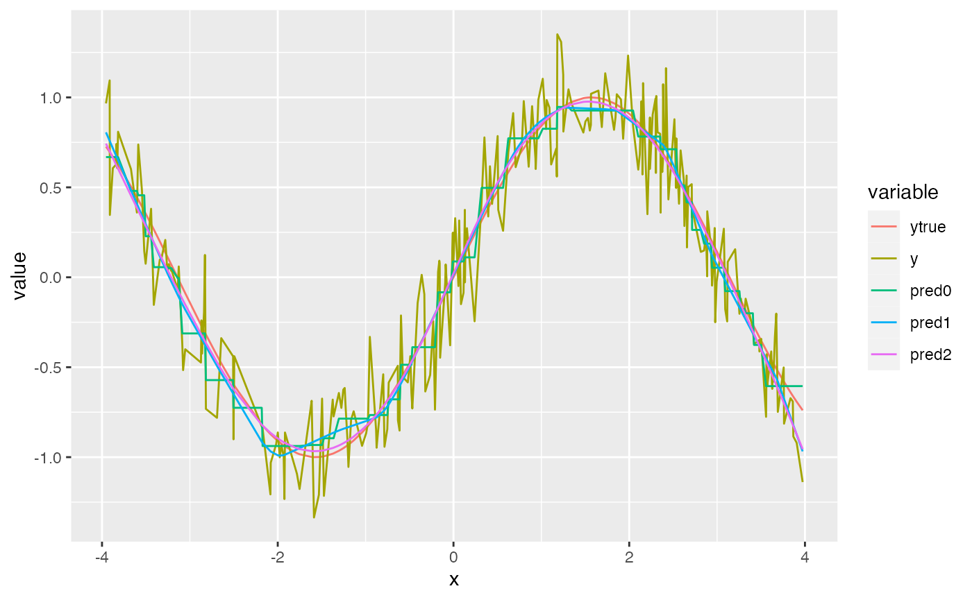
y <- sin(x[, 1]) + rnorm(n_obs, mean = 0, sd = 0.2)
ytrue <- sin(x[, 1])
hal_fit_0 <- fit_hal(
X = x, Y = y, smoothness_orders = 0, num_knots = num_knots
)
hal_fit_smooth_1 <- fit_hal(
X = x, Y = y, smoothness_orders = 1, num_knots = num_knots
)
hal_fit_smooth_2_all <- fit_hal(
X = x, Y = y, smoothness_orders = 2, num_knots = num_knots,
fit_control = list(cv_select = FALSE)
)
hal_fit_smooth_2 <- fit_hal(
X = x, Y = y, smoothness_orders = 2, num_knots = num_knots
)
pred_0 <- predict(hal_fit_0, new_data = x)
pred_smooth_1 <- predict(hal_fit_smooth_1, new_data = x)
pred_smooth_2 <- predict(hal_fit_smooth_2, new_data = x)
pred_smooth_2_all <- predict(hal_fit_smooth_2_all, new_data = x)
dt <- data.table(x = as.vector(x))
dt <- cbind(dt, pred_smooth_2_all)
long <- melt(dt, id = "x")
ggplot(long, aes(x = x, y = value, group = variable)) + geom_line()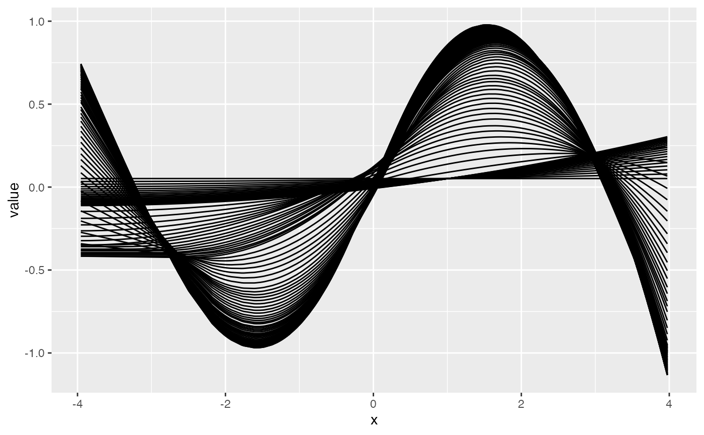
Comparing the mean squared error (MSE) between the predictions and
the true (denoised) outcome, the first- and second- order smoothed HAL
is able to recover from the coarseness of the basis functions caused by
the small num_knots argument. Also, the HAL with
second-order smoothness is able to fit the true function very well (as
expected, since sin(x) is a very smooth function). The main benefit of
imposing higher-order smoothness is that fewer knot points are required
for a near-optimal fit. Therefore, one can safely pass a smaller value
to num_knots for a big decrease in runtime without
sacrificing performance.
=======>>>>>>> 81093a5ceebcd36630f308dd07f69d4e30f07f1cmean((pred_0 - ytrue)^2)## [1] 0.00732315mean((pred_smooth_1- ytrue)^2)## [1] 0.003458005mean((pred_smooth_2 - ytrue)^2)## [1] 0.001834611dt <- data.table(x = as.vector(x), ytrue = ytrue, y = y, pred0 = pred_0, pred1 = pred_smooth_1, pred2 = pred_smooth_2) long <- melt(dt, id = "x") ggplot(long, aes(x = x, y = value, color = variable)) + geom_line()
plot(x, pred_0, main = "Zero order smoothness fit")
plot(x, pred_smooth_1, main = "First order smoothness fit")
plot(x, pred_smooth_2, main = "Second order smoothness fit")
In general, if the basis functions are not coarse, then the performance for different smoothness orders is similar. Notice how the runtime is a fair bit slower when more knot points are considered. In general, we recommend either zero- or first- order smoothness. Second-order smoothness tends to be less robust and suffers from extrapolation on new data. One can also use cross-validation to data-adaptively choose the optimal smoothness (invoked in
<<<<<<< HEADfit_halby settingadaptive_smoothing = TRUE). Comparing the following simulation and the previous one, the HAL with second-order smoothness performed better when there were fewer knot points.=======>>>>>>> 81093a5ceebcd36630f308dd07f69d4e30f07f1cset.seed(98109) n_covars <- 1 n_obs <- 250 x <- replicate(n_covars, runif(n_obs, min = -4, max = 4)) y <- sin(x[, 1]) + rnorm(n_obs, mean = 0, sd = 0.2) ytrue <- sin(x[, 1]) hal_fit_0 <- fit_hal( X = x, Y = y, smoothness_orders = 0, num_knots = 100 ) hal_fit_smooth_1 <- fit_hal( X = x, Y = y, smoothness_orders = 1, num_knots = 100 ) hal_fit_smooth_2 <- fit_hal( X = x, Y = y, smoothness_orders = 2, num_knots = 100 ) pred_0 <- predict(hal_fit_0, new_data = x) pred_smooth_1 <- predict(hal_fit_smooth_1, new_data = x) pred_smooth_2 <- predict(hal_fit_smooth_2, new_data = x)mean((pred_0 - ytrue)^2)## [1] 0.00732315mean((pred_smooth_1- ytrue)^2)## [1] 0.003458005mean((pred_smooth_2 - ytrue)^2)## [1] 0.001848927plot(x, pred_0, main = "Zero order smoothness fit")
plot(x, pred_smooth_1, main = "First order smoothness fit")
plot(x, pred_smooth_2, main = "Second order smoothness fit")
Formula interface
One might wish to specify the functional form of the HAL fit further. This can be done using the formula interface. Specifically, the formula interface allows one to specify monotonicity constraints on components of the HAL fit. It also allows one to specify exactly which basis functions (e.g., interactions) one wishes to model. The
<<<<<<< HEADformula_halfunction generates aformulaobject from a user-supplied character string, and thisformulaobject contains the necessary specification information forfit_halandglmnet. Theformula_halfunction is intended for use withinfit_hal, and the user-supplied character string is inputted intofit_hal. Here, we callformula_haldirectly for illustrative purposes.=======>>>>>>> 81093a5ceebcd36630f308dd07f69d4e30f07f1cset.seed(98109) num_knots <- 100 n_obs <- 500 x1 <- runif(n_obs, min = -4, max = 4) x2 <- runif(n_obs, min = -4, max = 4) A <- runif(n_obs, min = -4, max = 4) X <- data.frame(x1 = x1, x2 = x2, A = A) Y <- rowMeans(sin(X)) + rnorm(n_obs, mean = 0, sd = 0.2)We can specify an additive model in a number of ways.
The formula below includes the outcome, but
<<<<<<< HEADformula_haldoesn’t fit a HAL model, and doesn’t need the outcome (actually everything before “\(\tilde\)” is ignored informula_hal). This is whyformula_haltakes the inputXmatrix of covariates, and notXandY. In what follows, we include formulas with and without “y” in the character string.=======>>>>>>> 81093a5ceebcd36630f308dd07f69d4e30f07f1c# The `h` function is used to specify the basis functions for a given term # h(x1) generates one-way basis functions for the variable x1 # This is an additive model: formula <- ~h(x1) + h(x2) + h(A) #We can actually evaluate the h function as well. We need to specify some tuning parameters in the current environment: smoothness_orders <- 0 num_knots <- 10 # It will look in the parent environment for `X` and the above tuning parameters form_term <- h(x1) + h(x2) + h(A) form_term$basis_list[[1]]## $cols ## [1] 1 ## ## $cutoffs ## [1] -3.971502 ## ## $orders ## [1] 0# We don't need the variables in the parent environment if we specify them directly: rm(smoothness_orders) rm(num_knots) # `h` excepts the arguments `s` and `k`. `s` stands for smoothness and is equivalent to smoothness_orders in use. `k` specifies the number of knots. ` form_term_new <- h(x1, s = 0, k = 10) + h(x2, s = 0, k = 10) + h(A, s = 0, k = 10) # They are the same! length( form_term_new$basis_list) == length(form_term$basis_list)## [1] TRUE#To evaluate a unevaluated formula object like: formula <- ~h(x1) + h(x2) + h(A) # we can use the formula_hal function: formula <- formula_hal( ~ h(x1) + h(x2) + h(A), X = X, smoothness_orders = 1, num_knots = 10 ) # Note that the arguments smoothness_orders and/or num_knots will not be used if `s` and/or `k` are specified in `h`. formula <- formula_hal( Y ~ h(x1, k=1) + h(x2, k=1) + h(A, k=1), X = X, smoothness_orders = 1, num_knots = 10 )The
<<<<<<< HEAD.argument. We can generate an additive model for all or a subset of variables using the.variable and.argument ofh. By default,.inh(.)is treated as a wildcard and basis functions are generated by replacing the.with all variables inX.=======>>>>>>> 81093a5ceebcd36630f308dd07f69d4e30f07f1csmoothness_orders <- 1 num_knots <- 5 # A additive model colnames(X)## [1] "x1" "x2" "A"# Shortcut: formula1 <- h(.) # Longcut: formula2 <- h(x1) + h(x2) + h(A) # Same number of basis functions length(formula1$basis_list ) == length(formula2$basis_list)## [1] TRUE# Maybe we only want an additive model for x1 and x2 # Use the `.` argument formula1 <- h(., . = c("x1", "x2")) formula2 <- h(x1) + h(x2) length(formula1$basis_list ) == length(formula2$basis_list)## [1] TRUEWe can specify interactions as follows.
# Two way interactions formula1 <- h(x1) + h(x2) + h(A) + h(x1, x2) formula2 <- h(.) + h(x1, x2) length(formula1$basis_list ) == length(formula2$basis_list)## [1] TRUE# formula1 <- h(.) + h(x1, x2) + h(x1,A) + h(x2,A) formula2 <- h(.) + h(., .) length(formula1$basis_list ) == length(formula2$basis_list)## [1] TRUE# Three way interactions formula1 <- h(.) + h(.,.) + h(x1,A,x2) formula2 <- h(.) + h(., .)+ h(.,.,.) length(formula1$basis_list ) == length(formula2$basis_list)## [1] TRUESometimes, one might want to build an additive model, but include all two-way interactions with one variable (e.g., treatment “A”). This can be done in a variety of ways. The
<<<<<<< HEAD.argument allows you to specify a subset of variables.=======>>>>>>> 81093a5ceebcd36630f308dd07f69d4e30f07f1c# Write it all out formula <- h(x1) + h(x2) + h(A) + h(A, x1) + h(A,x2) # Use the "h(.)" which stands for add all additive terms and then manually add # interactions formula <- y ~ h(.) + h(A,x1) + h(A,x2) # Use the "wildcard" feature for when "." is included in the "h()" term. This # useful when you have many variables and do not want to write out every term. formula <- h(.) + h(A,.) formula1 <- h(A,x1) formula2 <- h(A,., . = c("x1")) length(formula1$basis_list) == length(formula2$basis_list)## [1] FALSEA key feature of the HAL formula is monotonicity constraints. Specifying these constraints is achieved by specifying the
<<<<<<< HEADmonotoneargument ofh. Note if smoothness_orders = 0 then this is a monotonicity constrain on the function, but if if smoothness_orders = 1 then this is a monotonicity constraint on the function’s derivative (e.g. a convexity constraint). We can also specify that certain terms are not penalized in the LASSO/glmnet using thepfargument ofh(stands for penalty factor).=======>>>>>>> 81093a5ceebcd36630f308dd07f69d4e30f07f1c# An additive monotone increasing model formula <- formula_hal( y ~ h(., monotone = "i"), X, smoothness_orders = 0, num_knots = 100 ) # An additive unpenalized monotone increasing model (NPMLE isotonic regressio) # Set the penalty factor argument `pf` to remove L1 penalization formula <- formula_hal( y ~ h(., monotone = "i", pf = 0), X, smoothness_orders = 0, num_knots = 100 ) # An additive unpenalized convex model (NPMLE convex regressio) # Set the penalty factor argument `pf` to remove L1 penalization # Note the second term is equivalent to adding unpenalized and unconstrained main-terms (e.g. main-term glm) formula <- formula_hal( ~ h(., monotone = "i", pf = 0, k=200, s=1) + h(., monotone = "none", pf = 0, k=1, s=1), X) # A bi-additive monotone decreasing model formula <- formula_hal( ~ h(., monotone = "d") + h(.,., monotone = "d"), X, smoothness_orders = 1, num_knots = 100 )The penalization feature can be used to reproduce glm
# Additive glm # One knot (at the origin) and first order smoothness formula <- h(., s = 1, k = 1, pf = 0) # Running HAL with this formula will be equivalent to running glm with the formula Y ~ . # intraction glm formula <- h(., ., s = 1, k = 1, pf = 0) + h(., s = 1, k = 1, pf = 0) # Running HAL with this formula will be equivalent to running glm with the formula Y ~ .^2Now, that we’ve illustrated the options with
<<<<<<< HEADformula_hal, let’s show how to fit a HAL model with the specified formula.=======>>>>>>> 81093a5ceebcd36630f308dd07f69d4e30f07f1c# get formula object fit <- fit_hal( X = X, Y = Y, formula = ~ h(.), smoothness_orders = 1, num_knots = 100 ) print(summary(fit), 10) # prints top 10 rows, i.e., highest absolute coefs## ## Summary of top 10 non-zero coefficients is based on lambda of 0.0005376299 ## ## coef term ## 0.7473715 (Intercept) ## -0.3081866 [ I(A >= -3.978)*(A - -3.978)^1 ] ## -0.2894577 [ I(x2 >= -3.992)*(x2 - -3.992)^1 ] ## -0.2811616 [ I(x1 >= 1.172)*(x1 - 1.172)^1 ] ## -0.2463477 [ I(x1 >= -3.972)*(x1 - -3.972)^1 ] ## -0.2405977 [ I(x2 >= 1.638)*(x2 - 1.638)^1 ] ## 0.2092225 [ I(x1 >= -1.45)*(x1 - -1.45)^1 ] ## 0.2078703 [ I(x2 >= -1.293)*(x2 - -1.293)^1 ] ## -0.2039605 [ I(A >= 1.384)*(A - 1.384)^1 ] ## 0.1993688 [ I(A >= -1.356)*(A - -1.356)^1 ]
References
Benkeser, David, and Mark J van der Laan. 2016. “The Highly Adaptive Lasso Estimator.” In 2016 IEEE International Conference on Data Science and Advanced Analytics (DSAA). IEEE. https://doi.org/10.1109/dsaa.2016.93.Coyle, Jeremy R, Nima S Hejazi, and Mark J van der Laan. n.d.hal9001: The Scalable Highly Adaptive Lasso (version 0.2.7). https://doi.org/10.5281/zenodo.3558313.Friedman, Jerome, Trevor Hastie, and Rob Tibshirani. 2010. “Regularization Paths for Generalized Linear Models via Coordinate Descent.” Journal of Statistical Software 33 (1): 1.Hejazi, Nima S, Jeremy R Coyle, and Mark J van der Laan. 2020. “hal9001: Scalable Highly Adaptive Lasso Regression in R.” Journal of Open Source Software 5 (53): 2526. https://doi.org/10.21105/joss.02526.van der Laan, Mark J. 2017. “Finite Sample Inference for Targeted Learning.” https://arxiv.org/abs/1708.09502.