7 Causal Mediation Analysis

Nima Hejazi

Based on the tmle3mediate R package.

7.1 Learning Objectives

Understand that you can estimate the natural direct and indirect effects for a binary treatment using the tmle3mediate R package.
Know where to learn more about the tmle3mediate package.

7.2 Causal Mediation Analysis

We only have time to briefly introduce these parameters. You can find more information in the relevant handbook chapter

In the presence of post-treatment intermediate variables affected by exposure (that is, mediators), path-specific effects allow for such complex, mechanistic relationships to be teased apart. These causal effects are of such wide interest that their definition and identification has been the object of study in statistics for nearly a century – indeed, the earliest examples of modern causal mediation analysis can be traced back to work on path analysis (???).

In recent decades, renewed interest has resulted in the formulation of novel direct and indirect effects within both the potential outcomes and nonparametric structural equation modeling frameworks (???; ???; ???; ???; Pearl 2009). Generally, the indirect effect (IE) is the portion of the total effect found to work through mediating variables, while the direct effect (DE) encompasses all other components of the total effect, including both the effect of the treatment directly on the outcome and its effect through all paths not explicitly involving the mediators. The mechanistic knowledge conveyed by the direct and indirect effects can be used to improve understanding of both why and how treatments may be efficacious.

7.3 Data Structure and Notation

Let us return to our familiar sample of \(n\) units \(O_1, \ldots, O_n\), where we now consider a slightly more complex data structure \(O = (W, A, Z, Y)\) for any given observational unit. As before, \(W\) represents a vector of observed covariates, \(A\) a binary or continuous treatment, and \(Y\) a binary or continuous outcome; the new post-treatment variable \(Z\) represents a (possibly multivariate) set of mediators. Avoiding assumptions unsupported by background scientific knowledge, we assume only that \(O \sim P_0 \in \M\), where \(\M\) is the nonparametric statistical model that places no assumptions on the form of the data-generating distribution \(P_0\).

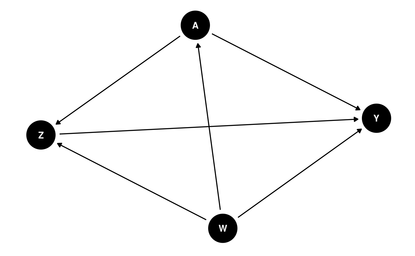
As in preceding chapters, a structural causal model (SCM) (Pearl 2009) helps to formalize the definition of our counterfactual variables: \[\begin{align} W &= f_W(U_W) \\ \nonumber A &= f_A(W, U_A) \\ \nonumber Z &= f_Z(W, A, U_Z) \\ \nonumber Y &= f_Y(W, A, Z, U_Y). \tag{7.1} \end{align}\] This set of equations constitutes a mechanistic model generating the observed data \(O\); furthermore, the SCM encodes several fundamental assumptions. Firstly, there is an implicit temporal ordering: \(W\) occurs first, depending only on exogenous factors \(U_W\); \(A\) happens next, based on both \(W\) and exogenous factors \(U_A\); then come the mediators \(Z\), which depend on \(A\), \(W\), and another set of exogenous factors \(U_Z\); and finally appears the outcome \(Y\). We assume neither access to the set of exogenous factors \(\{U_W, U_A, U_Z, U_Y\}\) nor knowledge of the forms of the deterministic generating functions \(\{f_W, f_A, f_Z, f_Y\}\). In practice, any available knowledge about the data-generating experiment should be incorporated into this model – for example, if the data from a randomized controlled trial (RCT), the form of \(f_A\) may be known. The SCM corresponds to the following DAG:

By factorizing the likelihood of the data \(O\), we can express \(p_0\), the density of \(O\) with respect to the product measure, when evaluated on a particular observation \(o\), in terms of several orthogonal components: \[\begin{align} p_0(o) = &q_{0,Y}(y \mid Z = z, A = a, W = w) \\ \nonumber &q_{0,Z}(z \mid A = a, W = w) \\ \nonumber &g_{0,A}(a \mid W = w) \\ \nonumber &q_{0,W}(w).\\ \nonumber \tag{7.2} \end{align}\] In Equation (7.2), \(q_{0, Y}\) is the conditional density of \(Y\) given \(\{Z, A, W\}\), \(q_{0, Z}\) is the conditional density of \(Z\) given \(\{A, W\}\), \(g_{0, A}\) is the conditional density of \(A\) given \(W\), and \(q_{0, W}\) is the marginal density of \(W\). For convenience and consistency of notation, we will define \(\overline{Q}_Y(Z, A, W) := \E[Y \mid Z, A, W]\) and \(g(A \mid W) := \P(A \mid W)\) (i.e., the propensity score).

7.4 Defining the Natural Direct and Indirect Effects

7.4.1 Decomposing the Average Treatment Effect

The natural direct and indirect effects arise from a decomposition of the ATE: \[\begin{align*} \E[Y(1) - Y(0)] = &\underbrace{\E[Y(1, Z(0)) - Y(0, Z(0))]}_{\text{NDE}} \\ &+ \underbrace{\E[Y(1, Z(1)) - Y(1, Z(0))]}_{\text{NIE}}. \end{align*}\] In particular, the natural indirect effect (NIE) measures the effect of the treatment \(A \in \{0, 1\}\) on the outcome \(Y\) through the mediators \(Z\), while the natural direct effect (NDE) measures the effect of the treatment on the outcome through all other pathways.

Identifiability results and necessary assumptions for these parameters are thoroughly covered in the handbook.

7.4.2 Estimating the Natural Direct Effect

The NDE is defined as \[\begin{align*} \psi_{\text{NDE}} =&~\E[Y(1, Z(0)) - Y(0, Z(0))] \\ =& \sum_w \sum_z [\underbrace{\E(Y \mid A = 1, z, w)}_{\overline{Q}_Y(A = 1, z, w)} - \underbrace{\E(Y \mid A = 0, z, w)}_{\overline{Q}_Y(A = 0, z, w)}] \\ &\times \underbrace{p(z \mid A = 0, w)}_{q_Z(Z \mid 0, w))} \underbrace{p(w)}_{q_W}, \end{align*}\] where the likelihood factors arise from a factorization of the joint likelihood: \[\begin{equation*} p(w, a, z, y) = \underbrace{p(y \mid w, a, z)}_{q_Y(A, W, Z)} \underbrace{p(z \mid w, a)}_{q_Z(Z \mid A, W)} \underbrace{p(a \mid w)}_{g(A \mid W)} \underbrace{p(w)}_{q_W}. \end{equation*}\]

The process of estimating the NDE begins by constructing \(\overline{Q}_{Y, n}\), an estimate of the conditional mean of the outcome, given \(Z\), \(A\), and \(W\). With an estimate of this conditional mean in hand, predictions of the quantities \(\overline{Q}_Y(Z, 1, W)\) (setting \(A = 1\)) and, likewise, \(\overline{Q}_Y(Z, 0, W)\) (setting \(A = 0\)) are readily obtained. We denote the difference of these conditional means \(\overline{Q}_{\text{diff}} = \overline{Q}_Y(Z, 1, W) - \overline{Q}_Y(Z, 0, W)\), which is itself only a functional parameter of the data distribution. \(\overline{Q}_{\text{diff}}\) captures differences in the conditional mean of \(Y\) across contrasts of \(A\).

A procedure for constructing a targeted maximum likelihood (TML) estimator of the NDE treats \(\overline{Q}_{\text{diff}}\) itself as a nuisance parameter, regressing its estimate \(\overline{Q}_{\text{diff}, n}\) on baseline covariates \(W\), among observations in the control condition only (i.e., those for whom \(A = 0\) is observed); the goal of this step is to remove part of the marginal impact of \(Z\) on \(\overline{Q}_{\text{diff}}\), since the covariates \(W\) precede the mediators \(Z\) in time. Regressing this difference on \(W\) among the controls recovers the expected \(\overline{Q}_{\text{diff}}\), under the setting in which all individuals are treated as falling in the control condition \(A = 0\). Any residual additive effect of \(Z\) on \(\overline{Q}_{\text{diff}}\) is removed during the TML estimation step using the auxiliary (or “clever”) covariate, which accounts for the mediators \(Z\). This auxiliary covariate takes the form

\[\begin{equation*} C_Y(q_Z, g)(O) = \Bigg\{\frac{\mathbb{I}(A = 1)}{g(1 \mid W)} \frac{q_Z(Z \mid 0, W)}{q_Z(Z \mid 1, W)} - \frac{\mathbb{I}(A = 0)}{g(0 \mid W)} \Bigg\} \ . \end{equation*}\] Breaking this down, \(\mathbb{I}(A = 1) / g(1 \mid W)\) is the inverse propensity score weight for \(A = 1\) and, likewise, \(\mathbb{I}(A = 0) / g(0 \mid W)\) is the inverse propensity score weight for \(A = 0\). The middle term is the ratio of the conditional densities of the mediator under the control (\(A = 0\)) and treatment (\(A = 1\)) conditions (n.b., recall the mediator positivity condition above).

This subtle appearance of a ratio of conditional densities is concerning – tools to estimate such quantities are sparse in the statistics literature (Dı́az and van der Laan 2011; Hejazi, Benkeser, and van der Laan 2020), unfortunately, and the problem is still more complicated (and computationally taxing) when \(Z\) is high-dimensional. As only the ratio of these conditional densities is required, a convenient re-parametrization may be achieved, that is, \[\begin{equation*} \frac{p(A = 0 \mid Z, W)}{g(0 \mid W)} \frac{g(1 \mid W)}{p(A = 1 \mid Z, W)} \ . \end{equation*}\] Going forward, we will denote this re-parameterized conditional probability functional \(e(A \mid Z, W) := p(A \mid Z, W)\). The same re-parameterization technique has been used by (???), (???), (???), (???), and (???) in similar contexts. This reformulation is particularly useful for the fact that it reduces the estimation problem to one requiring only the estimation of conditional means, opening the door to the use of a wide range of machine learning algorithms, as discussed previously.

Underneath the hood, the mean outcome difference \(\overline{Q}_{\text{diff}}\) and \(e(A \mid Z, W)\), the conditional probability of \(A\) given \(Z\) and \(W\), are used in constructing the auxiliary covariate for TML estimation. These nuisance parameters play an important role in the bias-correcting update step of the TML estimation procedure.

7.4.3 Estimating the Natural Indirect Effect

Derivation and estimation of the NIE is analogous to that of the NDE. Recall that the NIE is the effect of \(A\) on \(Y\) only through the mediator \(Z\). This counterfactual quantity, which may be expressed \(\E(Y(Z(1), 1) - \E(Y(Z(0), 1)\), corresponds to the difference of the conditional mean of \(Y\) given \(A = 1\) and \(Z(1)\) (the values the mediator would take under \(A = 1\)) and the conditional expectation of \(Y\) given \(A = 1\) and \(Z(0)\) (the values the mediator would take under \(A = 0\)).

As with the NDE, re-parameterization can be used to replace \(q_Z(Z \mid A, W)\) with \(e(A \mid Z, W)\) in the estimation process, avoiding estimation of a possibly multivariate conditional density. However, in this case, the mediated mean outcome difference, previously computed by regressing \(\overline{Q}_{\text{diff}}\) on \(W\) among the control units (for whom \(A = 0\) is observed) is instead replaced by a two-step process. First, \(\overline{Q}_Y(Z, 1, W)\), the conditional mean of \(Y\) given \(Z\) and \(W\) when \(A = 1\), is regressed on \(W\), among only the treated units (i.e., for whom \(A = 1\) is observed). Then, the same quantity, \(\overline{Q}_Y(Z, 1, W)\) is again regressed on \(W\), but this time among only the control units (i.e., for whom \(A = 0\) is observed). The mean difference of these two functionals of the data distribution is a valid estimator of the NIE. It can be thought of as the additive marginal effect of treatment on the conditional mean of \(Y\) given \((W, A = 1, Z)\) through its effect on \(Z\). So, in the case of the NIE, while our estimand \(\psi_{\text{NIE}}\) is different, the same estimation techniques useful for constructing efficient estimators of the NDE come into play.

7.5 The Population Intervention Direct and Indirect Effects

At times, the natural direct and indirect effects may prove too limiting, as these effect definitions are based on static interventions (i.e., setting \(A = 0\) or \(A = 1\)), which may be unrealistic for real-world interventions. In such cases, one may turn instead to the population intervention direct effect (PIDE) and the population intervention indirect effect (PIIE), which are based on decomposing the effect of the population intervention effect (PIE) of flexible stochastic interventions (???).

We previously discussed stochastic interventions when considering how to intervene on continuous-valued treatments; however, these intervention schemes may be applied to all manner of treatment variables. A particular type of stochastic intervention well-suited to working with binary treatments is the incremental propensity score intervention (IPSI), first proposed by (???). Such interventions do not deterministically set the treatment level of an observed unit to a fixed quantity (i.e., setting \(A = 1\)), but instead alter the odds of receiving the treatment by a fixed amount (\(0 \leq \delta \leq \infty\)) for each individual. In particular, this intervention takes the form \[\begin{equation*} g_{\delta}(1 \mid w) = \frac{\delta g(1 \mid w)}{\delta g(1 \mid w) + 1 - g(1\mid w)}, \end{equation*}\] where the scalar \(0 < \delta < \infty\) specifies a change in the odds of receiving treatment. As described by (???) in the context of causal mediation analysis, the identification assumptions required for the PIDE and the PIIE are significantly more lax than those required for the NDE and NIE. These identification assumptions include the following. Importantly, the assumption of cross-world counterfactual independence is not at all required.

Definition 7.1 (Conditional Exchangeability of Treatment and Mediators) Assume that \(\E\{Y(a, z) \mid Z, A, W\} = \E\{Y(a, z) \mid Z, W\}~\forall~(a, z) \in \mathcal{A} \times \mathcal{Z}W\). This assumption is stronger than and implied by the assumption \(Y(a, z) \indep (A,Z) \mid W\), originally proposed by (???) for identification of mediated effects among the treated. In introducing this assumption (???) state that “This assumption would be satisfied for any pre-exposure \(W\) in a randomized experiment in which exposure and mediators are randomized. Thus, the direct effect for a population intervention corresponds to contrasts between treatment regimes of a randomized experiment via interventions on \(A\) and \(Z\), unlike the natural direct effect for the average treatment effect (???).”

Definition 7.2 (Common Support of Treatment and Mediators) Assume that \(\text{supp}\{g_{\delta}(\cdot \mid w)\} \subseteq \text{supp}\{g(\cdot \mid w)\}~\forall~w \in \mathcal{W}\). This assumption is standard and requires only that the post-intervention value of \(A\) be supported in the data. Note that this is significantly weaker than the treatment and mediator positivity conditions required for the natural direct and indirect effects, and it is a direct consequence of using stochastic (rather than static) interventions.

7.6 Evaluating the Direct and Indirect Effects

We now turn to estimating the natural direct and indirect effects, as well as the population intervention direct effect, using the WASH Benefits data, introduced in earlier chapters. Let’s first load the data:

library(data.table)
library(sl3)
library(tmle3)
library(tmle3mediate)

# download data
washb_data <- fread(
  paste0(
    "https://raw.githubusercontent.com/tlverse/tlverse-data/master/",
    "wash-benefits/washb_data.csv"
  ),
  stringsAsFactors = TRUE
)

# make intervention node binary and subsample
washb_data <- washb_data[sample(.N, 600), ]
washb_data[, tr := as.numeric(tr != "Control")]

We’ll next define the baseline covariates \(W\), treatment \(A\), mediators \(Z\), and outcome \(Y\) nodes of the NPSEM via a “Node List” object:

node_list <- list(
  W = c(
    "momage", "momedu", "momheight", "hfiacat", "Nlt18", "Ncomp", "watmin",
    "elec", "floor", "walls", "roof"
  ),
  A = "tr",
  Z = c("sex", "month", "aged"),
  Y = "whz"
)

Here, the node_list encodes the parents of each node – for example, \(Z\) (the mediators) have parents \(A\) (the treatment) and \(W\) (the baseline confounders), and \(Y\) (the outcome) has parents \(Z\), \(A\), and \(W\). We’ll also handle any missingness in the data by invoking process_missing:

processed <- process_missing(washb_data, node_list)
washb_data <- processed$data
node_list <- processed$node_list

We’ll now construct an ensemble learner using a handful of popular machine learning algorithms:

# SL learners used for continuous data (the nuisance parameter Z)
enet_contin_learner <- Lrnr_glmnet$new(
  alpha = 0.5, family = "gaussian", nfolds = 3
)
lasso_contin_learner <- Lrnr_glmnet$new(
  alpha = 1, family = "gaussian", nfolds = 3
)
fglm_contin_learner <- Lrnr_glm_fast$new(family = gaussian())
mean_learner <- Lrnr_mean$new()
contin_learner_lib <- Stack$new(
  enet_contin_learner, lasso_contin_learner, fglm_contin_learner, mean_learner
)
sl_contin_learner <- Lrnr_sl$new(learners = contin_learner_lib)

# SL learners used for binary data (nuisance parameters G and E in this case)
enet_binary_learner <- Lrnr_glmnet$new(
  alpha = 0.5, family = "binomial", nfolds = 3
)
lasso_binary_learner <- Lrnr_glmnet$new(
  alpha = 1, family = "binomial", nfolds = 3
)
fglm_binary_learner <- Lrnr_glm_fast$new(family = binomial())
binary_learner_lib <- Stack$new(
  enet_binary_learner, lasso_binary_learner, fglm_binary_learner, mean_learner
)
sl_binary_learner <- Lrnr_sl$new(learners = binary_learner_lib)

# create list for treatment and outcome mechanism regressions
learner_list <- list(
  Y = sl_contin_learner,
  A = sl_binary_learner
)

7.6.1 Targeted Estimation of the Natural Indirect Effect

We demonstrate calculation of the NIE below, starting by instantiating a “Spec” object that encodes exactly which learners to use for the nuisance parameters \(e(A \mid Z, W)\) and \(\psi_Z\). We then pass our Spec object to the tmle3 function, alongside the data, the node list (created above), and a learner list indicating which machine learning algorithms to use for estimating the nuisance parameters based on \(A\) and \(Y\).

tmle_spec_NIE <- tmle_NIE(
  e_learners = Lrnr_cv$new(lasso_binary_learner, full_fit = TRUE),
  psi_Z_learners = Lrnr_cv$new(lasso_contin_learner, full_fit = TRUE),
  max_iter = 1
)
washb_NIE <- tmle3(
  tmle_spec_NIE, washb_data, node_list, learner_list
)
washb_NIE
A tmle3_Fit that took 1 step(s)
   type                  param  init_est  tmle_est       se     lower    upper
1:  NIE NIE[Y_{A=1} - Y_{A=0}] 0.0028004 0.0025696 0.043356 -0.082407 0.087546
   psi_transformed lower_transformed upper_transformed
1:       0.0025696         -0.082407          0.087546

Based on the output, we conclude that the indirect effect of the treatment through the mediators (sex, month, aged) is 0.00257.

7.6.2 Targeted Estimation of the Natural Direct Effect

An analogous procedure applies for estimation of the NDE, only replacing the Spec object for the NIE with tmle_spec_NDE to define learners for the NDE nuisance parameters:

tmle_spec_NDE <- tmle_NDE(
  e_learners = Lrnr_cv$new(lasso_binary_learner, full_fit = TRUE),
  psi_Z_learners = Lrnr_cv$new(lasso_contin_learner, full_fit = TRUE),
  max_iter = 1
)
washb_NDE <- tmle3(
  tmle_spec_NDE, washb_data, node_list, learner_list
)
washb_NDE
A tmle3_Fit that took 1 step(s)
   type                  param init_est tmle_est       se    lower   upper
1:  NDE NDE[Y_{A=1} - Y_{A=0}] 0.017372 0.017372 0.085844 -0.15088 0.18562
   psi_transformed lower_transformed upper_transformed
1:        0.017372          -0.15088           0.18562

From this, we can draw the conclusion that the direct effect of the treatment (through all paths not involving the mediators (sex, month, aged)) is 0.01737. Note that, together, the estimates of the natural direct and indirect effects approximately recover the average treatment effect, that is, based on these estimates of the NDE and NIE, the ATE is roughly 0.01994.

7.7 Exercises

Exercise 7.1 Examine the WASH Benefits dataset and choose a different set of potential mediators of the effect of the treatment on weight-for-height Z-score. Using this newly chosen set of mediators (or single mediator), estimate the natural direct and indirect effects. Provide an interpretation of these estimates.

Exercise 7.2 Assess whether additivity of the natural direct and indirect effects holds. Using the natural direct and indirect effects estimated above, does their sum recover the ATE?

Exercise 7.3 Evaluate whether the assumptions required for identification of the natural direct and indirect effects are plausible in the WASH Benefits example. In particular, position this evaluation in terms of empirical diagnostics of treatment and mediator positivity.

6 Stochastic Treatment Regimes (optional)

8 A Primer on the R6 Class System