5 Optimal Individualized Treatment Regimes

Ivana Malenica

Based on the tmle3mopttx R package by Ivana Malenica, Jeremy Coyle, and Mark van der Laan.

Updated: 2022-06-14

5.1 Learning Objectives

By the end of this lesson you will be able to:

Differentiate dynamic and optimal dynamic treatment interventions from static interventions.
Explain the benefits, and challenges, associated with using optimal individualized treatment regimes in practice.
Contrast the impact of implementing an optimal individualized treatment regime in the population with the impact of implementing static and dynamic treatment regimes in the population.
Estimate causal effects under optimal individualized treatment regimes with the tmle3mopttx R package.
Assess the mean under optimal individualized treatment with resource constraints.
Implement optimal individualized treatment rules based on sub-optimal rules, or “simple” rules, and recognize the practical benefit of these rules.
Construct “realistic” optimal individualized treatment regimes that respect real data and subject-matter knowledge limitations on interventions by only considering interventions that are supported by the data.
Measure variable importance as defined in terms of the optimal individualized treatment interventions.

5.2 Introduction

Identifying which intervention will be effective for which patient based on lifestyle, genetic and environmental factors is a common goal in precision medicine. One opts to administer the intervention to individuals who will benefit from it, instead of assigning treatment on a population level.

This aim motivates a different type of intervention, as opposed to the static exposures we might be used to.
In this chapter, we learn about dynamic (individualized) interventions that tailor the treatment decision based on the collected covariates.

To motivate these types of interventions, we turn to an actual randomized trial.

The goal is to improve retention in HIV care.
Several interventions show efficacy – appointment reminders through text messages, small cash incentives for on-time clinic visits, and peer health workers.
We want to improve effectiveness by assigning each patient the intervention they are most likely to benefit from.
We also do not want to allocate resources to individuals who would not benefit from an intervention.

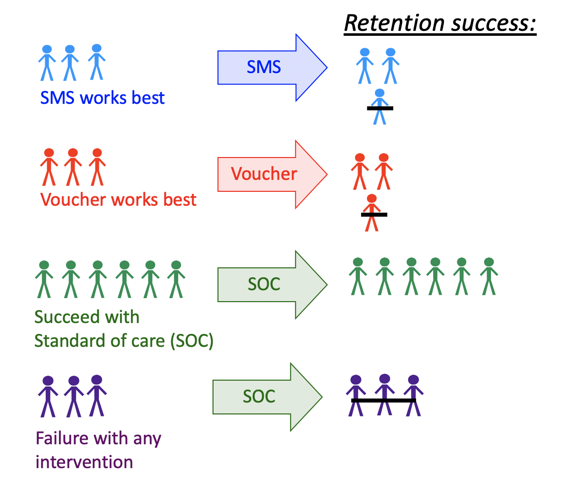
FIGURE 5.1: Illustration of a Dynamic Treatment Regime in a Clinical Setting

In the statistics community, such a treatment strategy is termed individualized treatment regimes (ITR). The (counterfactual) population mean outcome under an ITR is the value of the ITR.

Suppose one wishes to maximize the population mean of an outcome, where for each individual we have access to some set of measured covariates.
ITR with the maximal value is referred to as an optimal ITR or the optimal individualized treatment.
The value of an optimal ITR is termed the optimal value, or the mean under the optimal individualized treatment.
One opts to administer the intervention to individuals who will profit from it, instead of assigning treatment on a population level.

But how do we know which intervention works for which patient?

In this chapter, we examine optimal individualized treatment regimes, and estimate the mean outcome under the ITR.
The candidate rules are restricted to depend only on user-supplied subset of the baseline covariates.
We will use tmle3mopttx to estimate optimal ITR and the corresponding value.

5.3 Data Structure and Notation

Suppose we observe \(n\) independent and identically distributed observations of the form \(O=(W,A,Y) \sim P_0\).
\(P_0 \in \mathcal{M}\), where \(\mathcal{M}\) is the fully nonparametric model.
Denote \(A \in \mathcal{A}\) as categorical treatment.
Let \(\mathcal{A} \equiv \{a_1, \ldots, a_{n_A} \}\) and \(n_A = |\mathcal{A}|\), with \(n_A\) denoting the number of categories.
Denote \(Y\) as the final outcome.
\(W\) a vector-valued collection of baseline covariates.
Finally, let \(V\) be a subset of the baseline covariates \(W\) that the rule might depend on.

The likelihood of the data admits a factorization, implied by the time ordering of \(O\). \[\begin{align*}\label{eqn:likelihood_factorization} p_0(O) &= p_{Y,0}(Y|A,W) p_{A,0}(A|W) p_{W,0}(W) \\ &= q_{Y,0}(Y|A,W) q_{A,0}(A|W) q_{W,0}(W), \end{align*}\]
Consequently, let \[P_{Y,0}(Y|A,W)=Q_{Y,0}(Y|A,W),\] \[P_{A,0}(A|W)=g_0(A|W)\] and \[P_{W,0}(W)=Q_{W,0}(W).\]

We also define \(\bar{Q}_{Y,0}(A,W) \equiv E_0[Y|A,W]\).

5.4 Causal Effect of an OIT

We define relationships between variables with structural equations:

\[\begin{align*} W &= f_W(U_W) \\ A &= f_A(W, U_A) \\ Y &= f_Y(A, W, U_Y). \end{align*}\]

\(U=(U_W,U_A,U_Y)\) denotes the exogenous random variables, drawn from \(U \sim P_U\).
The endogenous variables, written as \(O=(W,A,Y)\), correspond to the observed data.

Causal effects are defined as hypothetical interventions on SEM.

Consider dynamic treatment rules, denoted as \(d\), in the set of all possible rules \(\mathcal{D}\).
In a point treatment setting, \(d\) is a deterministic function that takes as input \(V\) and outputs a treatment decision where

\[V \rightarrow d(V) \in \{a_1, \cdots, a_{n_A} \}.\]

For a given rule \(d\), our modified system then takes the following form:

\[\begin{align*} W &= f_W(U_W) \\ A &= d(V) \\ Y_{d(V)} &= f_Y(d(V), W, U_Y). \end{align*}\]

The counterfactual outcome \(Y_{d(V)}\) denotes the outcome for a patient had their treatment been assigned using the dynamic rule \(d(V)\) (possibly contrary to the fact).
Distribution of the counterfactual outcomes is \(P_{U,X}\), implied by the distribution of exogenous variables \(U\) and structural equations \(f\).
The set of all possible counterfactual distributions are encompassed by the causal model \(\mathcal{M}^F\), where \(P_{U,X} \in \mathcal{M}^F\).

“What is the expected outcome had every subject received treatment according to the (optimal) rule \(d\)?”

We can consider different treatment rules, all in the set \(\mathcal{D}\):

The true rule, \(d_0\), and the corresponding causal parameter \(E_{U,X}[Y_{d_0(V)}]\) denoting the expected outcome under the true treatment rule \(d_0(V)\).
The estimated rule, \(d_n\), and the corresponding causal parameter \(E_{U,X}[Y_{d_n(V)}]\) denoting the expected outcome under the estimated treatment rule \(d_n(V)\).

In this chapter, we will focus on the value under the estimated rule \(d_n\), a data-adaptive parameter.

Note that its true value depends on the sample!

The optimal individualized rule is the rule with the maximal value: \[d_{opt}(V) \equiv \text{argmax}_{d(V) \in \mathcal{D}} E_{P_{U,X}}[Y_{d(V)}].\]

Our causal target parameter of interest is the expected outcome under the estimated optimal individualized rule:

\[\Psi_{d_{n, \text{opt}}(V)}(P_{U,X}) := E_{P_{U,X}}[Y_{d_{n, \text{opt}}(V)}].\]

5.4.1 Identification and Statistical Estimand

In order for the causal quantities to be estimated from the observed data, they need to be identified with statistical parameters.

This step of the roadmap requires me make a few assumptions:

Strong ignorability: \(A\) independent of \(Y^{d_n(v)} \mid W\), for all \(a \in \mathcal{A}\).
Positivity (or overlap): \(P_0(\min_{a \in \mathcal{A}} g_0(a \mid W) > 0) = 1\)

Under the above causal assumptions, we can identify the causal target parameter with observed data using the G-computation formula.

The value of an individualized rule can now be expressed as

\[E_0[Y_{d_n(V)}] = E_{0,W}[\bar{Q}_{Y,0}(A=d_n(V),W)].\]

“Mean outcome if (possibly contrary to fact), treatment was assigned according to the rule \(d_n\).”

Finally, the statistical counterpart to the causal parameter of interest is defined as:

\[\psi_0 = E_{0,W}[\bar{Q}_{Y,0}(A=d_{n,\text{opt}}(V),W)].\]

“Mean outcome if (possibly contrary to fact), treatment was assigned according to the optimal rule \(d_{n,\text{opt}}\).”

5.4.2 High-level idea

Learn the optimal ITR using the Super Learner.

Estimate its value with the cross-validated Targeted Minimum Loss-based Estimator (CV-TMLE).

5.4.3 Why CV-TMLE?

CV-TMLE is necessary as the non-cross-validated TMLE is biased upward for the mean outcome under the rule, and therefore overly optimistic.
More generally however, using CV-TMLE allows us more freedom in estimation and therefore greater data adaptivity, without sacrificing inference.

5.5 Binary Treatment

How do we estimate the optimal individualized treatment regime?

In the case of binary treatment, a key quantity for optimal ITR is the blip function.
Optimal ITR assigns treatment to individuals falling in strata in which the stratum specific average treatment effect, the blip function, is positive.
Consequently, it does not assign treatment to individuals for which this quantity is negative.

We define the blip function as:

\[\bar{Q}_0(V) \equiv E_0[Y_1-Y_0|V] \equiv E_0[\bar{Q}_{Y,0}(1,W) - \bar{Q}_{Y,0}(0,W) | V], \] or the average treatment effect within a stratum of \(V\).

Optimal individualized rule can now be derived as: \[d_{opt}(V) = I(\bar{Q}_{0}(V) > 0).\]

We follow the below steps in order to obtain value of the ITR:

Estimate \(\bar{Q}_{Y,0}(A,W)\) and \(g_0(A|W)\) using sl3. We denote such estimates as \(\bar{Q}_{Y,n}(A,W)\) and \(g_n(A|W)\).

Apply the doubly robust Augmented-Inverse Probability Weighted (A-IPW) transform to our outcome, where we define:

\[D_{\bar{Q}_Y,g,a}(O) \equiv \frac{I(A=a)}{g(A|W)} (Y-\bar{Q}_Y(A,W)) + \bar{Q}_Y(A=a,W)\]

Few notes on the A-IPW transform:

Under the randomization and positivity assumptions, we have that \(E[D_{\bar{Q}_Y,g,a}(O) | V] = E[Y_a |V].\)
Due to the double robust nature of the A-IPW transform, consistency of \(E[Y_a |V]\) will depend on correct estimation of either \(\bar{Q}_{Y,0}(A,W)\) or \(g_0(A|W)\).
In a randomized trial, we are guaranteed a consistent estimate of \(E[Y_a |V]\) even if we get \(\bar{Q}_{Y,0}(A,W)\) wrong!

Using this transform, we can define the following contrast:

\[D_{\bar{Q}_Y,g}(O) = D_{\bar{Q}_Y,g,a=1}(O) - D_{\bar{Q}_Y,g,a=0}(O).\]

We estimate the blip function, \(\bar{Q}_{0,a}(V)\), by regressing \(D_{\bar{Q}_Y,g}(O)\) on \(V\).

Our estimated rule is \(d(V) = \text{argmax}_{a \in \mathcal{A}} \bar{Q}_{0,a}(V)\).

Finally, get the mean under the OIT:

We obtain inference for the mean outcome under the estimated optimal rule using CV-TMLE.

All combined:

Estimate \(\bar{Q}_{Y,0}(A,W)\) and \(g_0(A|W)\) using sl3. We denote such estimates as \(\bar{Q}_{Y,n}(A,W)\) and \(g_n(A|W)\).

Apply the doubly robust Augmented-Inverse Probability Weighted (A-IPW) transform to our outcome. Our estimated rule is \(d(V) = \text{argmax}_{a \in \mathcal{A}} \bar{Q}_{0,a}(V)\).

We obtain inference for the mean outcome under the estimated optimal rule using CV-TMLE.

5.5.1 Causal Effect of OIT with Binary A

To start, let us load the packages we will use and set a seed for simulation:

library(data.table)
library(sl3)
library(tmle3)
library(tmle3mopttx)
library(devtools)
library(here)
set.seed(111)

5.5.1.1 Simulate Data

Our data generating distribution is of the following form:

\[W \sim \mathcal{N}(\bf{0},I_{3 \times 3})\] \[P(A=1|W) = \frac{1}{1+\exp^{(-0.8*W_1)}}\]

\[\begin{align} P(Y=1|A,W) &= 0.5\text{logit}^{-1}[-5I(A=1)(W_1-0.5) \\ &+ 5I(A=0)(W_1-0.5)] +0.5\text{logit}^{-1}(W_2W_3) \end{align}\]

head(data)
          W1       W2       W3 A Y
1: -0.591031 -0.40168  0.15008 1 0
2:  0.026594 -0.37093  0.79472 0 0
3: -1.516553 -0.42515  0.43203 1 0
4: -1.362653  0.44115  0.34370 1 1
5:  1.178489 -0.67275  0.38710 1 0
6: -0.934151  0.41669 -0.78808 1 1

The above composes our observed data structure \(O = (W, A, Y)\).
Note that the mean under the OIT is \(\psi_0=0.578\) for this data generating distribution.

Next, we specify the role that each variable in the data set plays as the nodes in a DAG.

# organize data and nodes for tmle3
node_list <- list(
  W = c("W1", "W2", "W3"),
  A = "A",
  Y = "Y"
)
node_list
$W
[1] "W1" "W2" "W3"

$A
[1] "A"

$Y
[1] "Y"

We now have an observed data structure (data), and a specification of the role that each variable in the data set plays as the nodes in a DAG.

5.5.1.2 Constructing Stacked Regressions with `sl3`

We generate three different ensemble learners that must be fit.

learners for the outcome regression,
propensity score, and
blip function.

# Define sl3 library and metalearners:
lrn_mean  <- Lrnr_mean$new()
lrn_glm   <- Lrnr_glm_fast$new()
lrn_lasso <- Lrnr_glmnet$new()
lrnr_hal  <- Lrnr_hal9001$new(reduce_basis=1/sqrt(nrow(data)) )

## Define the Q learner:
Q_learner <- Lrnr_sl$new(
  learners = list(lrn_lasso, lrn_mean, lrn_glm),
  metalearner = Lrnr_nnls$new()
)

## Define the g learner:
g_learner <- Lrnr_sl$new(
  learners = list(lrn_lasso, lrn_glm),
  metalearner = Lrnr_nnls$new()
)

## Define the B learner:
b_learner <- Lrnr_sl$new(
  learners = list(lrn_mean, lrn_glm, lrn_lasso),
  metalearner = Lrnr_nnls$new()
)

We make the above explicit with respect to standard notation by bundling the ensemble learners into a list object below:

# specify outcome and treatment regressions and create learner list
learner_list <- list(Y = Q_learner, A = g_learner, B = b_learner)
learner_list
$Y
[1] "Super learner:"
List of 3
 $ : chr "Lrnr_glmnet_NULL_deviance_10_1_100_TRUE"
 $ : chr "Lrnr_mean"
 $ : chr "Lrnr_glm_fast_TRUE_Cholesky"

$A
[1] "Super learner:"
List of 2
 $ : chr "Lrnr_glmnet_NULL_deviance_10_1_100_TRUE"
 $ : chr "Lrnr_glm_fast_TRUE_Cholesky"

$B
[1] "Super learner:"
List of 3
 $ : chr "Lrnr_mean"
 $ : chr "Lrnr_glm_fast_TRUE_Cholesky"
 $ : chr "Lrnr_glmnet_NULL_deviance_10_1_100_TRUE"

5.5.1.3 Targeted Estimation

To start, we will initialize a specification for the TMLE of our parameter of interest simply by calling tmle3_mopttx_blip_revere.

We specify the argument V = c("W1", "W2", "W3") in order to communicate that we’re interested in learning a rule dependent on V covariates.
We also need to specify the type of blip we will use in this estimation problem, and the list of learners used.
In addition, we need to specify whether we want to maximize or minimize the mean outcome under the rule (maximize=TRUE).

# initialize a tmle specification
tmle_spec <- tmle3_mopttx_blip_revere(
  V = c("W1", "W2", "W3"), type = "blip1",
  learners = learner_list,
  maximize = TRUE, complex = TRUE,
  realistic = FALSE, resource = 1, 
  interpret=TRUE
)

# fit the TML estimator
fit <- tmle3(tmle_spec, data, node_list, learner_list)

# see the result
fit
A tmle3_Fit that took 1 step(s)
   type         param init_est tmle_est       se   lower   upper
1:  TSM E[Y_{A=NULL}]  0.35585  0.55755 0.025566 0.50744 0.60765
   psi_transformed lower_transformed upper_transformed
1:         0.55755           0.50744           0.60765

We can see that the confidence interval covers the truth!

We can also get the interpretable surrogate rule in terms of HAL:

# Interpretable rule
head(tmle_spec$blip_fit_interpret$coef)
[1]  0.368043  0.156435 -0.064386 -0.054062  0.042386  0.037879

# Interpretable rule
head(tmle_spec$blip_fit_interpret$term)
[1] "(Intercept)"                                                                                                  
[2] "[ I(W1 >= 0.899)*(W1 - 0.899)^1 ] * [ I(W2 >= -3.861)*(W2 - -3.861)^1 ]"                                      
[3] "[ I(W1 >= 0.074)*(W1 - 0.074)^1 ] * [ I(W2 >= -3.861)*(W2 - -3.861)^1 ] * [ I(W3 >= -2.945)*(W3 - -2.945)^1 ]"
[4] "[ I(W1 >= -1.418)*(W1 - -1.418)^1 ] * [ I(W2 >= -3.861)*(W2 - -3.861)^1 ]"                                    
[5] "[ I(W1 >= 0.856)*(W1 - 0.856)^1 ] * [ I(W2 >= -3.861)*(W2 - -3.861)^1 ] * [ I(W3 >= -1.292)*(W3 - -1.292)^1 ]"
[6] "[ I(W1 >= -1.368)*(W1 - -1.368)^1 ] * [ I(W2 >= -3.861)*(W2 - -3.861)^1 ] * [ I(W3 >= 0.843)*(W3 - 0.843)^1 ]"

5.5.1.4 Resource constraint

We can also restrict the number of individuals that get the treatment, even if giving treatment is beneficial (according to the estimated blip).

In order to impose a resource constraint, we have to specify the percent of individuals that will benefit the most from getting treatment.
For example, if resource=1, all individuals with blip higher than zero will get treatment.
If resource=0, none will get treatment.

# initialize a tmle specification
tmle_spec_resource <- tmle3_mopttx_blip_revere(
  V = c("W1", "W2", "W3"), type = "blip1",
  learners = learner_list,
  maximize = TRUE, complex = TRUE,
  realistic = FALSE, resource = 0.80
)

# fit the TML estimator
fit_resource <- tmle3(tmle_spec_resource, data, node_list, learner_list)

# see the result
fit_resource
A tmle3_Fit that took 1 step(s)
   type         param init_est tmle_est       se   lower   upper
1:  TSM E[Y_{A=NULL}]  0.32947  0.53611 0.025833 0.48548 0.58674
   psi_transformed lower_transformed upper_transformed
1:         0.53611           0.48548           0.58674

We can compare the number of individuals that got treatment with and without the resource constraint:

# Number of individuals with A=1 (no resource constraint):
table(tmle_spec$return_rule)

  0   1 
280 720 

# Number of individuals with A=1 (resource constraint):
table(tmle_spec_resource$return_rule)

  0   1 
422 578

5.5.1.5 Empty V

# initialize a tmle specification
tmle_spec_V_empty <- tmle3_mopttx_blip_revere(
  type = "blip1",
  learners = learner_list,
  maximize = TRUE, complex = TRUE,
  realistic = FALSE, resource = 1
)

# fit the TML estimator
fit_V_empty <- tmle3(tmle_spec_V_empty, data, node_list, learner_list)

# see the result:
fit_V_empty
A tmle3_Fit that took 1 step(s)
   type         param init_est tmle_est     se   lower   upper psi_transformed
1:  TSM E[Y_{A=NULL}]  0.32699  0.53301 0.0104 0.51263 0.55339         0.53301
   lower_transformed upper_transformed
1:           0.51263           0.55339

5.6 Categorical Treatment

QUESTION: What if the treatment is categorical, with more than two categories? Can we still use the blip function?

We define pseudo-blips: vector valued entities where the output for a given \(V\) is a vector of length equal to the number of treatment categories, \(n_A\).
As such, we define it as: \[\bar{Q}_0^{pblip}(V) = \{\bar{Q}_{0,a}^{pblip}(V): a \in \mathcal{A} \}.\]

We implement three different pseudo-blips in tmle3mopttx.

Blip1 corresponds to choosing a reference category of treatment, and defining the blip for all other categories relative to the specified reference: \[\bar{Q}_{0,a}^{pblip-ref}(V) \equiv E_0(Y_a-Y_0|V)\]
Blip2 corresponds to defining the blip relative to the average of all categories: \[\bar{Q}_{0,a}^{pblip-avg}(V) \equiv E_0(Y_a- \frac{1}{n_A} \sum_{a \in \mathcal{A}} Y_a|V)\]
Blip3 reflects an extension of Blip2, where the average is now a weighted average: \[\bar{Q}_{0,a}^{pblip-wavg}(V) \equiv E_0(Y_a- \frac{1}{n_A} \sum_{a \in \mathcal{A}} Y_{a} P(A=a|V) |V)\]

5.6.1 Causal Effect of OIT with Categorical A

We now need to pay attention to the type of blip we define in the estimation stage, as well as how we construct our learners.

5.6.1.1 Simulated Data

First, we load the simulated data. Here, our data generating distribution was of the following form:

\[W \sim \mathcal{N}(\bf{0},I_{4 \times 4})\] \[P(A|W) = \frac{1}{1+\exp^{(-(0.05*I(A=1)*W_1+0.8*I(A=2)*W_1+0.8*I(A=3)*W_1))}}\]

\[P(Y|A,W)=0.5\text{logit}^{-1}[15I(A=1)(W_1-0.5) - 3I(A=2)(2W_1+0.5) \\ + 3I(A=3)(3W_1-0.5)] +\text{logit}^{-1}(W_2W_1)\]

We can just load the data available as part of the package as follows:

head(data)
   W1       W2       W3       W4 A Y
1:  2 -0.40168  0.15008  1.44274 2 1
2:  3 -0.37093  0.79472  1.08879 3 0
3:  1 -0.42515  0.43203  0.22471 2 1
4:  1  0.44115  0.34370  1.55538 3 0
5:  3 -0.67275  0.38710 -0.31411 2 0
6:  1  0.41669 -0.78808 -0.28718 2 1

The above constructs our observed data structure \(O = (W, A, Y)\).
The true mean under the OIT is \(\psi=0.658\), which is the quantity we aim to estimate.

# organize data and nodes for tmle3
data <- data_cat_realistic
node_list <- list(
  W = c("W1", "W2", "W3", "W4"),
  A = "A",
  Y = "Y"
)
node_list
$W
[1] "W1" "W2" "W3" "W4"

$A
[1] "A"

$Y
[1] "Y"

We can see the number of observed categories of treatment below:

# organize data and nodes for tmle3
table(data$A)

  1   2   3 
 24 528 448

5.6.1.2 Constructing Stacked Regressions with `sl3`

QUESTION: With categorical treatment, what is the dimension of the blip now? What is the dimension for the current example? How would we go about estimating it?

# Initialize few of the learners:
lrn_xgboost_50 <- Lrnr_xgboost$new(nrounds = 50)
lrn_mean <- Lrnr_mean$new()
lrn_glm <- Lrnr_glm_fast$new()

## Define the Q learner, which is just a regular learner:
Q_learner <- Lrnr_sl$new(
  learners = list(lrn_xgboost_50, lrn_mean, lrn_glm),
  metalearner = Lrnr_nnls$new()
)

## Define the g learner, which is a multinomial learner:
# specify the appropriate loss of the multinomial learner:
mn_metalearner <- make_learner(Lrnr_solnp,
  eval_function = loss_loglik_multinomial,
  learner_function = metalearner_linear_multinomial
)
g_learner <- make_learner(Lrnr_sl, list(lrn_xgboost_50, lrn_mean), mn_metalearner)

## Define the Blip learner, which is a multivariate learner:
learners <- list(lrn_xgboost_50, lrn_mean, lrn_glm)
b_learner <- create_mv_learners(learners = learners)

We need to estimate \(g_0(A|W)\) for a categorical \(A\): we use the multinomial Super Learner option available within the sl3 package.
We need to estimate the blip using a multivariate Super Learner available within the sl3 package.

In order to see which learners can be used to estimate \(g_0(A|W)\) in sl3, we run the following:

# See which learners support multi-class classification:
sl3_list_learners(c("categorical"))
 [1] "Lrnr_bound"                "Lrnr_caret"               
 [3] "Lrnr_cv_selector"          "Lrnr_ga"                  
 [5] "Lrnr_glmnet"               "Lrnr_grf"                 
 [7] "Lrnr_gru_keras"            "Lrnr_h2o_glm"             
 [9] "Lrnr_h2o_grid"             "Lrnr_independent_binomial"
[11] "Lrnr_lightgbm"             "Lrnr_lstm_keras"          
[13] "Lrnr_mean"                 "Lrnr_multivariate"        
[15] "Lrnr_nnet"                 "Lrnr_optim"               
[17] "Lrnr_polspline"            "Lrnr_pooled_hazards"      
[19] "Lrnr_randomForest"         "Lrnr_ranger"              
[21] "Lrnr_rpart"                "Lrnr_screener_correlation"
[23] "Lrnr_solnp"                "Lrnr_svm"                 
[25] "Lrnr_xgboost"

# specify outcome and treatment regressions and create learner list
learner_list <- list(Y = Q_learner, A = g_learner, B = b_learner)
learner_list
$Y
[1] "Super learner:"
List of 3
 $ : chr "Lrnr_xgboost_50_1"
 $ : chr "Lrnr_mean"
 $ : chr "Lrnr_glm_fast_TRUE_Cholesky"

$A
[1] "Super learner:"
List of 2
 $ : chr "Lrnr_xgboost_50_1"
 $ : chr "Lrnr_mean"

$B
[1] "Super learner:"
List of 3
 $ : chr "Lrnr_xgboost_50_1_multivariate"
 $ : chr "Lrnr_mean_multivariate"
 $ : chr "Lrnr_glm_fast_TRUE_Cholesky_multivariate"

5.6.1.3 Targeted Estimation

# initialize a tmle specification
tmle_spec_cat <- tmle3_mopttx_blip_revere(
  V = c("W1", "W2", "W3", "W4"), type = "blip2",
  learners = learner_list, maximize = TRUE, complex = TRUE,
  realistic = FALSE
)

# fit the TML estimator
fit_cat <- tmle3(tmle_spec_cat, data, node_list, learner_list)

# see the result:
fit_cat
A tmle3_Fit that took 1 step(s)
   type         param init_est tmle_est       se   lower   upper
1:  TSM E[Y_{A=NULL}]  0.54334  0.61973 0.063746 0.49479 0.74467
   psi_transformed lower_transformed upper_transformed
1:         0.61973           0.49479           0.74467

# How many individuals got assigned each treatment?
table(tmle_spec_cat$return_rule)

  1   2   3 
438 380 182

We can see that the confidence interval covers the truth.

NOTICE the distribution of the assigned treatment! We will need this shortly.

5.7 Extensions

We consider multiple extensions to the procedure described for estimating the value of the ITR.

One might be interested in a grid of possible suboptimal rules, corresponding to potentially limited knowledge of potential effect modifiers (Simpler Rules).

Certain regimes might be preferred, but due to positivity restraints are not realistic to implement (Realistic Interventions).

5.7.1 Simpler Rules

We define \(S\)-optimal rules as the optimal rule that considers all possible subsets of \(V\) covariates, with card(\(S\)) \(\leq\) card(\(V\)) and \(\emptyset \in S\).

This allows us to consider sub-optimal rules that are easier to estimate: we allow for statistical inference for the counterfactual mean outcome under the sub-optimal rule.

# initialize a tmle specification
tmle_spec_cat_simple <- tmle3_mopttx_blip_revere(
  V = c("W4", "W3", "W2", "W1"), type = "blip2",
  learners = learner_list,
  maximize = TRUE, complex = FALSE, realistic = FALSE
)

# fit the TML estimator
fit_cat_simple <- tmle3(tmle_spec_cat_simple, data, node_list, learner_list)

# see the result:
fit_cat_simple
A tmle3_Fit that took 1 step(s)
   type                param init_est tmle_est      se   lower   upper
1:  TSM E[Y_{d(V=W3,W2,W1)}]  0.55423  0.62196 0.05204 0.51997 0.72396
   psi_transformed lower_transformed upper_transformed
1:         0.62196           0.51997           0.72396

Even though the user specified all baseline covariates as the basis for rule estimation, a simpler rule is sufficient to maximize the mean under the optimal individualized treatment.

QUESTION: How does the set of covariates picked by tmle3mopttx compare to the baseline covariates the true rule depends on?

5.7.2 Realistic Optimal Individual Regimes

tmle3mopttx also provides an option to estimate the mean under the realistic, or implementable, optimal individualized treatment.

It is often the case that assigning particular regime might optimize the desired outcome, but due to global or practical positivity constrains, such treatment can never be implemented (or is highly unlikely).
Specifying realistic="TRUE", we consider possibly suboptimal treatments that optimize the outcome in question while being supported by the data.

# initialize a tmle specification
tmle_spec_cat_realistic <- tmle3_mopttx_blip_revere(
  V = c("W4", "W3", "W2", "W1"), type = "blip2",
  learners = learner_list,
  maximize = TRUE, complex = TRUE, realistic = TRUE
)

# fit the TML estimator
fit_cat_realistic <- tmle3(tmle_spec_cat_realistic, data, node_list, learner_list)

# see the result:
fit_cat_realistic
A tmle3_Fit that took 1 step(s)
   type         param init_est tmle_est       se  lower   upper psi_transformed
1:  TSM E[Y_{A=NULL}]   0.5546  0.57351 0.059035 0.4578 0.68921         0.57351
   lower_transformed upper_transformed
1:            0.4578           0.68921

# How many individuals got assigned each treatment?
table(tmle_spec_cat_realistic$return_rule)

  1   2   3 
  5 511 484

QUESTION: Referring back to the data-generating distribution, why do you think the distribution of allocated treatment changed from the distribution we had under the “non-realistic”" rule?

5.7.3 Missingness and `tmle3mopttx`

In this section, we present how to use the tmle3mopttx package when the data is subject to missingness. Currently we support missing process on the following nodes:

outcome node, \(Y\);

all other types of missingness are handled by sl3 package. Let’s add some missingness to our outcome.

data_missing <- data_cat_realistic

#Add some random missingless:
rr <- sample(nrow(data_missing), 100, replace = FALSE)
data_missing[rr,"Y"]<-NA

# look at the data again:
summary(data_missing$Y)
   Min. 1st Qu.  Median    Mean 3rd Qu.    Max.    NA's 
   0.00    0.00    0.00    0.47    1.00    1.00     100

To start, we must first add to our library.

delta_learner <- Lrnr_sl$new(
  learners = list(lrn_mean, lrn_glm),
  metalearner = Lrnr_nnls$new()
)

# specify outcome and treatment regressions and create learner list
learner_list <- list(Y = Q_learner, A = g_learner, B = b_learner, delta_Y=delta_learner)
learner_list
$Y
[1] "Super learner:"
List of 3
 $ : chr "Lrnr_xgboost_50_1"
 $ : chr "Lrnr_mean"
 $ : chr "Lrnr_glm_fast_TRUE_Cholesky"

$A
[1] "Super learner:"
List of 2
 $ : chr "Lrnr_xgboost_50_1"
 $ : chr "Lrnr_mean"

$B
[1] "Super learner:"
List of 3
 $ : chr "Lrnr_xgboost_50_1_multivariate"
 $ : chr "Lrnr_mean_multivariate"
 $ : chr "Lrnr_glm_fast_TRUE_Cholesky_multivariate"

$delta_Y
[1] "Super learner:"
List of 2
 $ : chr "Lrnr_mean"
 $ : chr "Lrnr_glm_fast_TRUE_Cholesky"

Now delta_Y fits the missing outcome process.

# initialize a tmle specification
tmle_spec_cat_miss <- tmle3_mopttx_blip_revere(
  V = c("W1", "W2", "W3", "W4"), type = "blip2",
  learners = learner_list, maximize = TRUE, complex = TRUE,
  realistic = FALSE
)

# fit the TML estimator
fit_cat_miss <- tmle3(tmle_spec_cat_miss, data_missing, node_list, learner_list)

fit_cat_miss
A tmle3_Fit that took 1 step(s)
   type                    param init_est tmle_est       se   lower   upper
1:  TSM E[Y_{A=NULL, delta_Y=1}]  0.55533  0.81095 0.017859 0.77595 0.84595
   psi_transformed lower_transformed upper_transformed
1:         0.81095           0.77595           0.84595

5.7.4 Variable Importance Analysis

In order to run tmle3mopttx variable importance measure, we need to considered covariates that are categorical variables.

For illustration purpose, we bin baseline covariates corresponding to the data-generating distribution described in the previous section:

# bin baseline covariates to 3 categories:
data$W1<-ifelse(data$W1<quantile(data$W1)[2],1,ifelse(data$W1<quantile(data$W1)[3],2,3))

node_list <- list(
  W = c("W3", "W4", "W2"),
  A = c("W1", "A"),
  Y = "Y"
)
node_list
$W
[1] "W3" "W4" "W2"

$A
[1] "W1" "A" 

$Y
[1] "Y"

Note that our node list now includes \(W_1\) as treatments as well!
Don’t worry, we will still properly adjust for all baseline covariates when considering \(A\) as treatment.

5.7.4.1 Targeted Estimation

We will initialize a specification for the TMLE of our parameter of interest (called a tmle3_Spec in the tlverse nomenclature) simply by calling tmle3_mopttx_vim.

# initialize a tmle specification
tmle_spec_vim <- tmle3_mopttx_vim(
  V=c("W2"),
  type = "blip2",
  learners = learner_list,
  maximize = FALSE,
  method = "SL",
  complex = TRUE,
  realistic = FALSE
)

# fit the TML estimator
vim_results <- tmle3_vim(tmle_spec_vim, data, node_list, learner_list,
  adjust_for_other_A = TRUE
)

# see results:
print(vim_results)
   type                param   init_est  tmle_est       se      lower
1:  ATE E[Y_{A=NULL}] - E[Y] -0.0128837 -0.051833 0.021934 -0.0948231
2:  ATE E[Y_{A=NULL}] - E[Y] -0.0022747  0.036924 0.017144  0.0033228
        upper psi_transformed lower_transformed upper_transformed  A
1: -0.0088424       -0.051833        -0.0948231        -0.0088424 W1
2:  0.0705248        0.036924         0.0033228         0.0705248  A
             W  Z_stat      p_nz p_nz_corrected
1:  W3,W4,W2,A -2.3631 0.0090615       0.015629
2: W3,W4,W2,W1  2.1538 0.0156285       0.015629

The final result of tmle3_vim with the tmle3mopttx spec is an ordered list of mean outcomes under the optimal individualized treatment for all categorical covariates in our dataset.

5.8 Exercise

5.8.1 Real World Data and `tmle3mopttx`

Finally, we cement everything we learned so far with a real data application.

As in the previous sections, we will be using the WASH Benefits data, corresponding to the effect of water quality, sanitation, hand washing, and nutritional interventions on child development in rural Bangladesh trial.

The main aim of the cluster-randomized controlled trial was to assess the impact of six intervention groups, including:

Control
Handwashing with soap
Improved nutrition through counselling and provision of lipid-based nutrient supplements
Combined water, sanitation, handwashing, and nutrition.
Improved sanitation
Combined water, sanitation, and handwashing
Chlorinated drinking water

We aim to estimate the optimal ITR and the corresponding value under the optimal ITR for the main intervention in WASH Benefits data.

Our outcome of interest is the weight-for-height Z-score, whereas our treatment is the six intervention groups aimed at improving living conditions.

Questions:

Define \(V\) as mother’s education (momedu), current living conditions (floor), and possession of material items including the refrigerator (asset_refrig). Do we want to minimize or maximize the outcome? Which blip type should we use? Construct an appropriate sl3 library for \(A\), \(Y\) and \(B\).
Based on the \(V\) defined in the previous question, estimate the mean under the ITR for the main randomized intervention used in the WASH Benefits trial with weight-for-height Z-score as the outcome. What’s the TMLE value of the optimal ITR? How does it change from the initial estimate? Which intervention is the most dominant? Why do you think that is?
Using the same formulation as in questions 1 and 2, estimate the realistic optimal ITR and the corresponding value of the realistic ITR. Did the results change? Which intervention is the most dominant under realistic rules? Why do you think that is?

5.8.2 Solutions

To start, let’s load the data, convert all columns to be of class numeric, and take a quick look at it:

washb_data <- fread("https://raw.githubusercontent.com/tlverse/tlverse-data/master/wash-benefits/washb_data.csv", stringsAsFactors = TRUE)
washb_data <- washb_data[!is.na(momage), lapply(.SD, as.numeric)]
head(washb_data, 3)

As before, we specify the NPSEM via the node_list object.

node_list <- list(W = names(washb_data)[!(names(washb_data) %in% c("whz", "tr", "momheight"))],
                  A = "tr", Y = "whz")

We pick few potential effect modifiers, including mother’s education, current living conditions (floor), and possession of material items including the refrigerator. We concentrate of these covariates as they might be indicative of the socio-economic status of individuals involved in the trial. We can explore the distribution of our \(V\), \(A\) and \(Y\):

#V1, V2 and V3:
table(washb_data$momedu)
table(washb_data$floor)
table(washb_data$asset_refrig)

#A:
table(washb_data$tr)

#Y:
summary(washb_data$whz)

We specify a simple library for the outcome regression, propensity score and the blip function. Since our treatment is categorical, we need to define a multinomial learner for \(A\) and multivariate learner for \(B\). We will define the xgboost over a grid of parameters, and initialize a mean learner.

# Initialize few of the learners:
grid_params = list(nrounds = c(100, 500),
                     eta = c(0.01, 0.1))
grid = expand.grid(grid_params, KEEP.OUT.ATTRS = FALSE)
xgb_learners = apply(grid, MARGIN = 1, function(params_tune) {
    do.call(Lrnr_xgboost$new, c(as.list(params_tune)))
  })
lrn_mean <- Lrnr_mean$new()

## Define the Q learner, which is just a regular learner:
Q_learner <- Lrnr_sl$new(
  learners = list(xgb_learners[[1]], xgb_learners[[2]], xgb_learners[[3]],
                  xgb_learners[[4]], lrn_mean),
  metalearner = Lrnr_nnls$new()
)

## Define the g learner, which is a multinomial learner:
#specify the appropriate loss of the multinomial learner:
mn_metalearner <- make_learner(Lrnr_solnp, loss_function = loss_loglik_multinomial,
                               learner_function = metalearner_linear_multinomial)
g_learner <- make_learner(Lrnr_sl, list(xgb_learners[[4]], lrn_mean), mn_metalearner)

## Define the Blip learner, which is a multivariate learner:
learners <- list(xgb_learners[[1]], xgb_learners[[2]], xgb_learners[[3]],
                  xgb_learners[[4]], lrn_mean)
b_learner <- create_mv_learners(learners = learners)

learner_list <- list(Y = Q_learner, A = g_learner, B = b_learner)

As seen before, we initialize the tmle3_mopttx_blip_revere Spec in order to answer Question 1. We want to maximize our outcome, with higher the weight-for-height Z-score the better. We will also use blip2 as the blip type, but note that we could have used blip1 as well since “Control” is a good reference category.

## Question 2:

#Initialize a tmle specification
tmle_spec_Q <- tmle3_mopttx_blip_revere(
  V = c("momedu", "floor", "asset_refrig"), type = "blip2",
  learners = learner_list, maximize = TRUE, complex = TRUE,
  realistic = FALSE
)

#Fit the TML estimator.
fit_Q <- tmle3(tmle_spec_Q, data=washb_data, node_list, learner_list)
fit_Q

#Which intervention is the most dominant? 
table(tmle_spec_Q$return_rule)

Using the same formulation as before, we estimate the realistic optimal ITR and the corresponding value of the realistic ITR:

## Question 3:

#Initialize a tmle specification with "realistic=TRUE":
tmle_spec_Q_realistic <- tmle3_mopttx_blip_revere(
  V = c("momedu", "floor", "asset_refrig"), type = "blip2",
  learners = learner_list, maximize = TRUE, complex = TRUE,
  realistic = TRUE
)

#Fit the TML estimator.
fit_Q_realistic <- tmle3(tmle_spec_Q_realistic, data=washb_data, node_list, learner_list)
fit_Q_realistic

table(tmle_spec_Q_realistic$return_rule)

4 The TMLE Framework

6 Stochastic Treatment Regimes