5.1 Learning Objectives

By the end of this lesson you will be able to:

1. Differentiate dynamic and optimal dynamic treatment interventions from static interventions.
2. Explain the benefits and challenges associated with using optimal individualized treatment regimes in practice.
3. Contrast the impact of implementing an optimal individualized treatment regime in the population with the impact of implementing static and dynamic treatment regimes in the population.
4. Estimate causal effects under optimal individualized treatment regimes with the tmle3mopttx R package.
5. Implement optimal individualized treatment rules based on sub-optimal rules, or “simple” rules, and recognize the practical benefit of these rules.
6. Construct “realistic” optimal individualized treatment regimes that respect real data and subject-matter knowledge limitations on interventions by only considering interventions that are supported by the data.
7. Measure variable importance as defined in terms of the optimal individualized treatment interventions.

5.2 Introduction to Optimal Individualized Interventions

Identifying which intervention will be effective for which patient based on lifestyle, genetic and environmental factors is a common goal in precision medicine. One opts to administer the intervention to individuals who will benefit from it, instead of assigning treatment on a population level.

• This aim motivates a different type of an intervention, as opposed to the static exposures we might be used to.

• In this chapter, we learn about dynamic (individualized) interventions that tailor the treatment decision based on the collected covariates.

• In the statistics community, such a treatment strategy is termed individualized treatment regimes (ITR), and the (counterfactual) population mean outcome under an ITR is the value of the ITR.

• Even more, suppose one wishes to maximize the population mean of an outcome, where for each individual we have access to some set of measured covariates. An ITR with the maximal value is referred to as an optimal ITR or the optimal individualized treatment. Consequently, the value of an optimal ITR is termed the optimal value, or the mean under the optimal individualized treatment.

• One opts to administer the intervention to individuals who will profit from it, instead of assigning treatment on a population level. But how do we know which intervention works for which patient?

• For example, one might seek to improve retention in HIV care. In a randomized clinical trial, several interventions show efficacy- including appointment reminders through text messages, small cash incentives for on time clinic visits, and peer health workers.

• Ideally, we want to improve effectiveness by assigning each patient the intervention they are most likely to benefit from, as well as improve efficiency by not allocating resources to individuals that do not need them, or would not benefit from an intervention.

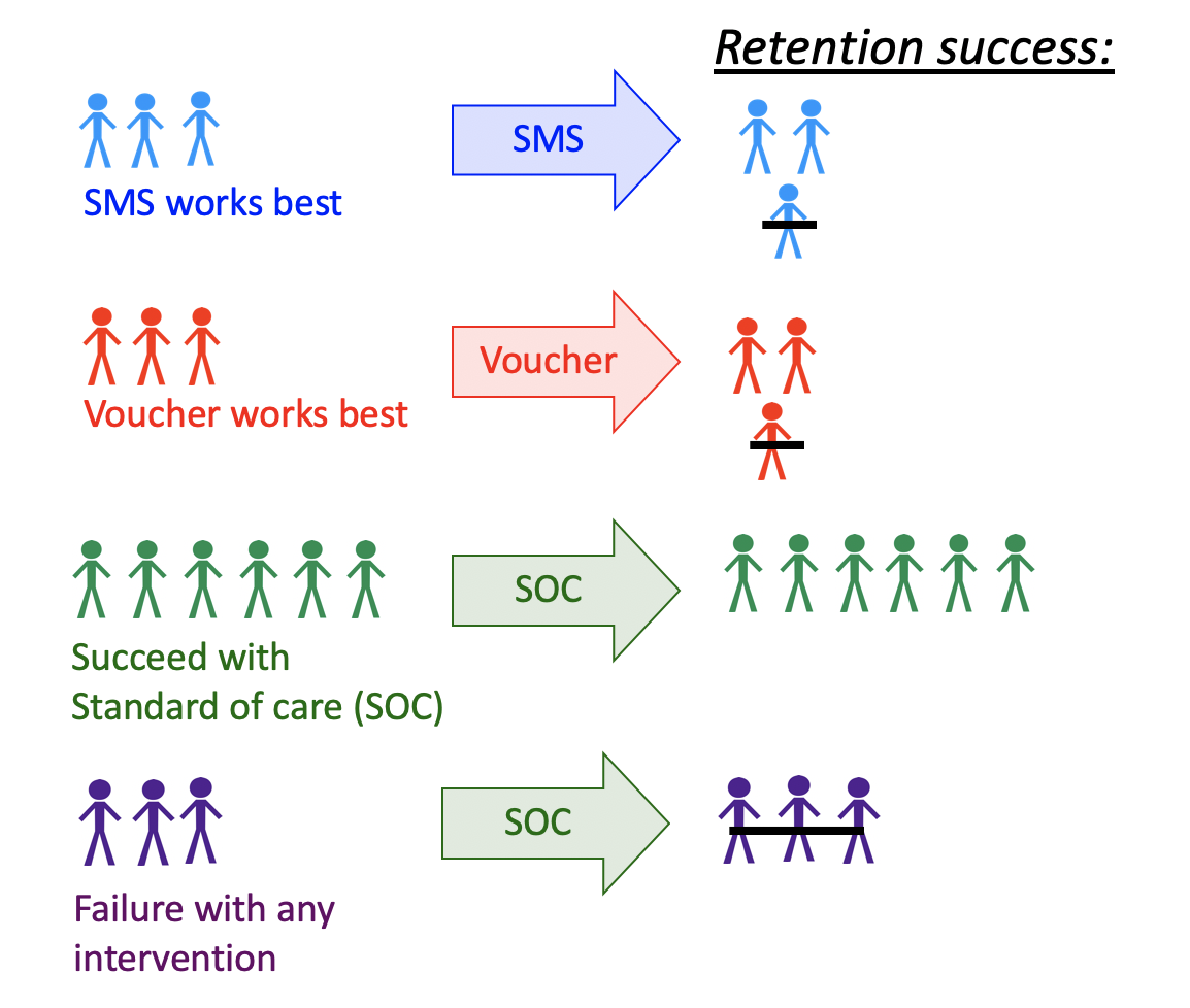
FIGURE 5.1: Illustration of a Dynamic Treatment Regime in a Clinical Setting

This aim motivates a different type of intervention, as opposed to the static exposures we might be used to.

• In this chapter, we examine multiple examples of optimal individualized treatment regimes and estimate the mean outcome under the ITR where the candidate rules are restricted to depend only on user-supplied subset of the baseline covariates.

• In order to accomplish this, we present the tmle3mopttx R package, which features an implementation of a recently developed algorithm for computing targeted minimum loss-based estimates of a causal effect based on optimal ITR for categorical treatment.

• In particular, we will use tmle3mopttx to estimate optimal ITR and the corresponding population value, construct realistic optimal ITRs, and perform variable importance in terms of the mean under the optimal individualized treatment.

5.3 Data Structure and Notation

• Suppose we observe \(n\) independent and identically distributed observations of the form \(O=(W,A,Y) \sim P_0\). \(P_0 \in \mathcal{M}\), where \(\mathcal{M}\) is the fully nonparametric model.

• Denote \(A \in \mathcal{A}\) as categorical treatment, where \(\mathcal{A} \equiv \{a_1, \ldots, a_{n_A} \}\) and \(n_A = |\mathcal{A}|\), with \(n_A\) denoting the number of categories.

• Denote \(Y\) as the final outcome, and \(W\) a vector-valued collection of baseline covariates.

• The likelihood of the data admits a factorization, implied by the time ordering of \(O\). \[\begin{equation*}\label{eqn:likelihood_factorization} p_0(O) = p_{Y,0}(Y|A,W) p_{A,0}(A|W) p_{W,0}(W) = q_{Y,0}(Y|A,W) q_{A,0}(A|W) q_{W,0}(W), \end{equation*}\]

• Consequently, we define \(P_{Y,0}(Y|A,W)=Q_{Y,0}(Y|A,W)\), \(P_{A,0}(A|W)=g_0(A|W)\) and \(P_{W,0}(W)=Q_{W,0}(W)\) as the corresponding conditional distributions of \(Y\), \(A\) and \(W\).

• We also define \(\bar{Q}_{Y,0}(A,W) \equiv E_0[Y|A,W]\).

• Finally, denote \(V\) as a subset of the baseline covariates \(W\) that the optimal individualized rule depends on.

5.4 Defining the Causal Effect of an Optimal Individualized Intervention

• Consider dynamic treatment rules \(V \rightarrow d(V) \in \{a_1, \ldots, a_{n_A} \} \times \{1\}\), for assigning treatment \(A\) based on \(V\).

• Dynamic treatment regime may be viewed as an intervention in which \(A\) is set equal to a value based on a hypothetical regime \(d(V)\), and \(Y_{d(V)}\) is the corresponding counterfactual outcome under \(d(V)\).

• The goal of any causal analysis motivated by an optimal individualized intervention is to estimate a parameter defined as the counterfactual mean of the outcome with respect to the modified intervention distribution.

• Recall causal assumptions:

1. Consistency: \(Y^{d(v_i)}_i = Y_i\) in the event \(A_i = d(v_i)\), for \(i = 1, \ldots, n\).
2. Stable unit value treatment assumption (SUTVA): \(Y^{d(v_i)}_i\) does not depend on \(d(v_j)\) for \(i = 1, \ldots, n\) and \(j \neq i\), or lack of interference.
3. Strong ignorability: \(A \perp \!\!\! \perp Y^{d(v)} \mid W\), for all \(a \in \mathcal{A}\).
4. Positivity (or overlap): \(P_0(\min_{a \in \mathcal{A}} g_0(a|W) > 0)=1\)

• Here, we also assume non-exceptional law is in effect.

• We are primarily interested in the value of an individualized rule, \[E_0[Y_{d(V)}] = E_{0,W}[\bar{Q}_{Y,0}(A=d(V),W)].\]

• The optimal rule is the rule with the maximal value: \[d_{opt}(V) \equiv \text{argmax}_{d(V) \in \mathcal{D}} E_0[Y_{d(V)}] \] where \(\mathcal{D}\) represents the set of possible rules, \(d\), implied by \(V\).

• The target causal estimand of our analysis is: \[\psi_0 := E_0[Y_{d_{opt}(V)}] = E_{0,W}[\bar{Q}_{Y,0}(A=d_{opt}(V),W)].\]

• General, high-level idea:

1. Learn the optimal ITR using the Super Learner.

2. Estimate its value with the cross-validated Targeted Minimum Loss-based Estimator (CV-TMLE).

5.5 Binary Treatment

• How do we estimate the optimal individualized treatment regime? In the case of a binary treatment, a key quantity for optimal ITR is the blip function.

• Optimal ITR ideally assigns treatment to individuals falling in strata in which the stratum specific average treatment effect, the blip function, is positive and does not assign treatment to individuals for which this quantity is negative.

• We define the blip function as: \[\bar{Q}_0(V) \equiv E_0[Y_1-Y_0|V] \equiv E_0[\bar{Q}_{Y,0}(1,W) - \bar{Q}_{Y,0}(0,W) | V], \] or the average treatment effect within a stratum of \(V\).

• Optimal individualized rule can now be derived as \(d_{opt}(V) = I(\bar{Q}_{0}(V) > 0)\).

• Relying on the Targeted Maximum Likelihood (TML) estimator and the Super Learner estimate of the blip function, we follow the below steps in order to obtain value of the ITR:

1. Estimate \(\bar{Q}_{Y,0}(A,W)\) and \(g_0(A|W)\) using sl3. We denote such estimates as \(\bar{Q}_{Y,n}(A,W)\) and \(g_n(A|W)\).

2. Apply the doubly robust Augmented-Inverse Probability Weighted (A-IPW) transform to our outcome, where we define:

\[D_{\bar{Q}_Y,g,a}(O) \equiv \frac{I(A=a)}{g(A|W)} (Y-\bar{Q}_Y(A,W)) + \bar{Q}_Y(A=a,W)\]

Note that under the randomization and positivity assumptions we have that \(E[D_{\bar{Q}_Y,g,a}(O) | V] = E[Y_a |V].\) We emphasize the double robust nature of the A-IPW transform: consistency of \(E[Y_a |V]\) will depend on correct estimation of either \(\bar{Q}_{Y,0}(A,W)\) or \(g_0(A|W)\). As such, in a randomized trial, we are guaranteed a consistent estimate of \(E[Y_a |V]\) even if we get \(\bar{Q}_{Y,0}(A,W)\) wrong!

Using this transform, we can define the following contrast:

\[D_{\bar{Q}_Y,g}(O) = D_{\bar{Q}_Y,g,a=1}(O) - D_{\bar{Q}_Y,g,a=0}(O)\]

We estimate the blip function, \(\bar{Q}_{0,a}(V)\), by regressing \(D_{\bar{Q}_Y,g}(O)\) on \(V\) using the specified sl3 library of learners and an appropriate loss function.

3. Our estimated rule is \(d(V) = \text{argmax}_{a \in \mathcal{A}} \bar{Q}_{0,a}(V)\).

4. We obtain inference for the mean outcome under the estimated optimal rule using CV-TMLE.

library(here)
library(data.table)
library(sl3)
library(tmle3)
library(tmle3mopttx)
library(devtools)
set.seed(116)

data("data_bin")

# organize data and nodes for tmle3
data <- data_bin
node_list <- list(
  W = c("W1", "W2", "W3"),
  A = "A",
  Y = "Y"
)

# Define sl3 library and metalearners:
lrn_xgboost_50 <- Lrnr_xgboost$new(nrounds = 50)
lrn_xgboost_100 <- Lrnr_xgboost$new(nrounds = 100)
lrn_xgboost_500 <- Lrnr_xgboost$new(nrounds = 500)
lrn_mean <- Lrnr_mean$new()
lrn_glm <- Lrnr_glm_fast$new()

## Define the Q learner:
Q_learner <- Lrnr_sl$new(
  learners = list(
    lrn_xgboost_50, lrn_xgboost_100,
    lrn_xgboost_500, lrn_mean, lrn_glm
  ),
  metalearner = Lrnr_nnls$new()
)

## Define the g learner:
g_learner <- Lrnr_sl$new(
  learners = list(lrn_xgboost_100, lrn_glm),
  metalearner = Lrnr_nnls$new()
)

## Define the B learner:
b_learner <- Lrnr_sl$new(
  learners = list(
    lrn_xgboost_50, lrn_xgboost_100,
    lrn_xgboost_500, lrn_mean, lrn_glm
  ),
  metalearner = Lrnr_nnls$new()
)

# specify outcome and treatment regressions and create learner list
learner_list <- list(Y = Q_learner, A = g_learner, B = b_learner)

# initialize a tmle specification
tmle_spec <- tmle3_mopttx_blip_revere(
  V = c("W1", "W2", "W3"), type = "blip1",
  learners = learner_list,
  maximize = TRUE, complex = TRUE,
  realistic = FALSE
)

# fit the TML estimator
fit <- tmle3(tmle_spec, data, node_list, learner_list)
fit
#> A tmle3_Fit that took 1 step(s)
#>    type         param init_est tmle_est       se   lower   upper
#> 1:  TSM E[Y_{A=NULL}]  0.43164  0.55855 0.027047 0.50554 0.61156
#>    psi_transformed lower_transformed upper_transformed
#> 1:         0.55855           0.50554           0.61156

5.6 Categorical Treatment

QUESTION: Can we still use the blip function if the treatment is categorical?

• In this section, we consider how to evaluate the mean outcome under the optimal individualized treatment when \(A\) has more than two categories!

• We define pseudo-blips as vector valued entities where the output for a given \(V\) is a vector of length equal to the number of treatment categories, \(n_A\). As such, we define it as: \[\bar{Q}_0^{pblip}(V) = \{\bar{Q}_{0,a}^{pblip}(V): a \in \mathcal{A} \}\]

• We implement three different pseudo-blips in tmle3mopttx.

1. Blip1 corresponds to choosing a reference category of treatment, and defining the blip for all other categories relative to the specified reference: \[\bar{Q}_{0,a}^{pblip-ref}(V) \equiv E_0(Y_a-Y_0|V)\]

2. Blip2 approach corresponds to defining the blip relative to the average of all categories: \[\bar{Q}_{0,a}^{pblip-avg}(V) \equiv E_0(Y_a- \frac{1}{n_A} \sum_{a \in \mathcal{A}} Y_a|V)\]

3. Blip3 reflects an extension of Blip2, where the average is now a weighted average: \[\bar{Q}_{0,a}^{pblip-wavg}(V) \equiv E_0(Y_a- \frac{1}{n_A} \sum_{a \in \mathcal{A}} Y_{a} P(A=a|V) |V)\]

data("data_cat_realistic")

# organize data and nodes for tmle3
data <- data_cat_realistic
node_list <- list(
  W = c("W1", "W2", "W3", "W4"),
  A = "A",
  Y = "Y"
)

# Initialize few of the learners:
lrn_xgboost_50 <- Lrnr_xgboost$new(nrounds = 50)
lrn_xgboost_100 <- Lrnr_xgboost$new(nrounds = 100)
lrn_xgboost_500 <- Lrnr_xgboost$new(nrounds = 500)
lrn_mean <- Lrnr_mean$new()
lrn_glm <- Lrnr_glm_fast$new()

## Define the Q learner, which is just a regular learner:
Q_learner <- Lrnr_sl$new(
  learners = list(lrn_xgboost_50, lrn_xgboost_100, lrn_xgboost_500, lrn_mean, lrn_glm),
  metalearner = Lrnr_nnls$new()
)

# Define the g learner, which is a multinomial learner:
# specify the appropriate loss of the multinomial learner:
mn_metalearner <- make_learner(Lrnr_solnp,
  loss_function = loss_loglik_multinomial,
  learner_function = metalearner_linear_multinomial
)
g_learner <- make_learner(Lrnr_sl, list(lrn_xgboost_100, lrn_xgboost_500, lrn_mean), mn_metalearner)

# Define the Blip learner, which is a multivariate learner:
learners <- list(lrn_xgboost_50, lrn_xgboost_100, lrn_xgboost_500, lrn_mean, lrn_glm)
b_learner <- create_mv_learners(learners = learners)

# See which learners support multi-class classification:
sl3_list_learners(c("categorical"))
#>  [1] "Lrnr_bound"                "Lrnr_caret"               
#>  [3] "Lrnr_cv_selector"          "Lrnr_glmnet"              
#>  [5] "Lrnr_grf"                  "Lrnr_gru_keras"           
#>  [7] "Lrnr_h2o_glm"              "Lrnr_h2o_grid"            
#>  [9] "Lrnr_independent_binomial" "Lrnr_lightgbm"            
#> [11] "Lrnr_lstm_keras"           "Lrnr_mean"                
#> [13] "Lrnr_multivariate"         "Lrnr_nnet"                
#> [15] "Lrnr_optim"                "Lrnr_polspline"           
#> [17] "Lrnr_pooled_hazards"       "Lrnr_randomForest"        
#> [19] "Lrnr_ranger"               "Lrnr_rpart"               
#> [21] "Lrnr_screener_correlation" "Lrnr_solnp"               
#> [23] "Lrnr_svm"                  "Lrnr_xgboost"

# specify outcome and treatment regressions and create learner list
learner_list <- list(Y = Q_learner, A = g_learner, B = b_learner)

# initialize a tmle specification
tmle_spec <- tmle3_mopttx_blip_revere(
  V = c("W1", "W2", "W3", "W4"), type = "blip2",
  learners = learner_list, maximize = TRUE, complex = TRUE,
  realistic = FALSE
)

# fit the TML estimator
fit <- tmle3(tmle_spec, data, node_list, learner_list)
fit
#> A tmle3_Fit that took 1 step(s)
#>    type         param init_est tmle_est       se   lower   upper
#> 1:  TSM E[Y_{A=NULL}]  0.54158  0.65915 0.068054 0.52577 0.79254
#>    psi_transformed lower_transformed upper_transformed
#> 1:         0.65915           0.52577           0.79254

# How many individuals got assigned each treatment?
table(tmle_spec$return_rule)
#> 
#>   1   2   3 
#> 428 394 178

5.7 Extensions to Causal Effect of an OIT

• We consider two extensions to the procedure described for estimating the value of the ITR.

• The first one considers a setting where the user might be interested in a grid of possible suboptimal rules, corresponding to potentially limited knowledge of potential effect modifiers (Simpler Rules).

• The second extension concerns implementation of realistic optimal individual interventions where certain regimes might be preferred, but due to practical or global positivity restraints are not realistic to implement (Realistic Interventions).

# initialize a tmle specification
tmle_spec <- tmle3_mopttx_blip_revere(
  V = c("W4", "W3", "W2", "W1"), type = "blip2",
  learners = learner_list,
  maximize = TRUE, complex = FALSE, realistic = FALSE
)

# fit the TML estimator
fit <- tmle3(tmle_spec, data, node_list, learner_list)
fit
#> A tmle3_Fit that took 1 step(s)
#>    type      param init_est tmle_est       se   lower   upper psi_transformed
#> 1:  TSM E[Y_{A=1}]  0.48614  0.53913 0.093273 0.35632 0.72194         0.53913
#>    lower_transformed upper_transformed
#> 1:           0.35632           0.72194

# initialize a tmle specification
tmle_spec <- tmle3_mopttx_blip_revere(
  V = c("W4", "W3", "W2", "W1"), type = "blip2",
  learners = learner_list,
  maximize = TRUE, complex = TRUE, realistic = TRUE
)

# fit the TML estimator
fit <- tmle3(tmle_spec, data, node_list, learner_list)
fit
#> A tmle3_Fit that took 1 step(s)
#>    type         param init_est tmle_est       se   lower   upper
#> 1:  TSM E[Y_{A=NULL}]  0.54869  0.58779 0.057258 0.47557 0.70001
#>    psi_transformed lower_transformed upper_transformed
#> 1:         0.58779           0.47557           0.70001

# How many individuals got assigned each treatment?
table(tmle_spec$return_rule)
#> 
#>   1   2   3 
#>   4 502 494

# bin baseline covariates to 3 categories:
data$W1 <- ifelse(data$W1 < quantile(data$W1)[2], 1, ifelse(data$W1 < quantile(data$W1)[3], 2, 3))

node_list <- list(
  W = c("W3", "W4", "W2"),
  A = c("W1", "A"),
  Y = "Y"
)

# initialize a tmle specification
tmle_spec <- tmle3_mopttx_vim(
  V = c("W2"),
  type = "blip2",
  learners = learner_list,
  contrast = "multiplicative",
  maximize = FALSE,
  method = "SL",
  complex = TRUE,
  realistic = FALSE
)

# fit the TML estimator
vim_results <- tmle3_vim(tmle_spec, data, node_list, learner_list,
  adjust_for_other_A = TRUE
)

print(vim_results)
#>    type                  param   init_est  tmle_est       se      lower
#> 1:   RR RR(E[Y_{A=NULL}]/E[Y])  0.0052065  0.058406 0.034144 -0.0085144
#> 2:   RR RR(E[Y_{A=NULL}]/E[Y]) -0.0239991 -0.067511 0.051592 -0.1686303
#>       upper psi_transformed lower_transformed upper_transformed  A           W
#> 1: 0.125327         1.06015           0.99152            1.1335  A W3,W4,W2,W1
#> 2: 0.033608         0.93472           0.84482            1.0342 W1  W3,W4,W2,A
#>     Z_stat     p_nz p_nz_corrected
#> 1:  1.7106 0.043578       0.087156
#> 2: -1.3085 0.095344       0.095344

5.8 Exercise

5.9 Summary

• In summary, the mean outcome under the optimal individualized treatment is a counterfactual quantity of interest representing what the mean outcome would have been if everybody, contrary to the fact, received treatment that optimized their outcome.

• tmle3mopttx estimates the mean outcome under the optimal individualized treatment, where the candidate rules are restricted to only respond to a user-supplied subset of the baseline and intermediate covariates. In addition it provides options for realistic, data-adaptive interventions.

• In essence, our target parameter answers the key aim of precision medicine: allocating the available treatment by tailoring it to the individual characteristics of the patient, with the goal of optimizing the final outcome.

washb_data <- fread("https://raw.githubusercontent.com/tlverse/tlverse-data/master/wash-benefits/washb_data.csv", stringsAsFactors = TRUE)
washb_data <- washb_data[!is.na(momage), lapply(.SD, as.numeric)]
head(washb_data, 3)

node_list <- list(
  W = names(washb_data)[!(names(washb_data) %in% c("whz", "tr"))],
  A = "tr", Y = "whz"
)

# V1, V2 and V3:
table(washb_data$momedu)
table(washb_data$floor)
table(washb_data$asset_refrig)

# A:
table(washb_data$tr)

# Y:
summary(washb_data$whz)

# Initialize few of the learners:
grid_params <- list(
  nrounds = c(100, 500),
  eta = c(0.01, 0.1)
)
grid <- expand.grid(grid_params, KEEP.OUT.ATTRS = FALSE)
xgb_learners <- apply(grid, MARGIN = 1, function(params_tune) {
  do.call(Lrnr_xgboost$new, c(as.list(params_tune)))
})
lrn_mean <- Lrnr_mean$new()

## Define the Q learner, which is just a regular learner:
Q_learner <- Lrnr_sl$new(
  learners = list(
    xgb_learners[[1]], xgb_learners[[2]], xgb_learners[[3]],
    xgb_learners[[4]], lrn_mean
  ),
  metalearner = Lrnr_nnls$new()
)

# Define the g learner, which is a multinomial learner:
# specify the appropriate loss of the multinomial learner:
mn_metalearner <- make_learner(Lrnr_solnp,
  loss_function = loss_loglik_multinomial,
  learner_function = metalearner_linear_multinomial
)
g_learner <- make_learner(Lrnr_sl, list(xgb_learners[[4]], lrn_mean), mn_metalearner)

# Define the Blip learner, which is a multivariate learner:
learners <- list(
  xgb_learners[[1]], xgb_learners[[2]], xgb_learners[[3]],
  xgb_learners[[4]], lrn_mean
)
b_learner <- create_mv_learners(learners = learners)

learner_list <- list(Y = Q_learner, A = g_learner, B = b_learner)

## Question 2:

# Initialize a tmle specification
tmle_spec <- tmle3_mopttx_blip_revere(
  V = c("momedu", "floor", "asset_refrig"), type = "blip2",
  learners = learner_list, maximize = TRUE, complex = TRUE,
  realistic = FALSE
)

# Fit the TML estimator.
fit <- tmle3(tmle_spec, data = washb_data, node_list, learner_list)
fit

# Which intervention is the most dominant?
table(tmle_spec$return_rule)

## Question 3:

# Initialize a tmle specification with "realistic=TRUE":
tmle_spec <- tmle3_mopttx_blip_revere(
  V = c("momedu", "floor", "asset_refrig"), type = "blip2",
  learners = learner_list, maximize = TRUE, complex = TRUE,
  realistic = TRUE
)

# Fit the TML estimator.
fit <- tmle3(tmle_spec, data = washb_data, node_list, learner_list)
fit

table(tmle_spec$return_rule)