10 Causal Mediation Analysis

Nima Hejazi

Featuring the tmle3mediate R package.

Learning Objectives

1. Examine how the presence of post-treatment mediating variables can complicate a causal analysis, and how direct and indirect effects can be defined to resolve these complications.
2. Describe the essential similarities and differences between direct and indirect causal effects, including their definition in terms of stochastic interventions.
3. Differentiate the joint interventions required to define direct and indirect effects from the static, dynamic, and stochastic interventions that yield total causal effects.
4. Describe the assumptions needed for identification of the natural direct and indirect effects, as well as the limitations of these effect definitions.
5. Estimate the natural direct and indirect effects for a binary treatment using the tmle3mediate R package.
6. Differentiate the population intervention direct and indirect effects of stochastic interventions from the natural direct and indirect effects, including differences in the assumptions required for their identification.
7. Estimate the population intervention direct effect of a binary treatment using the tmle3mediate R package.

10.1 Causal Mediation Analysis

In applications ranging from biology and epidemiology to economics and psychology, scientific inquires are often concerned with ascertaining the effect of a treatment on an outcome variable only through particular pathways between the two. In the presence of post-treatment intermediate variables affected by exposure (that is, mediators), path-specific effects allow for such complex, mechanistic relationships to be teased apart. These causal effects are of such wide interest that their definition and identification has been the object of study in statistics for nearly a century – indeed, the earliest examples of modern causal mediation analysis can be traced back to work on path analysis (Wright, 1934). In recent decades, renewed interest has resulted in the formulation of novel direct and indirect effects within both the potential outcomes and nonparametric structural equation modeling frameworks (Dawid, 2000; Pearl, 1995, 2009; JM Robins, 1986; Spirtes et al., 2000). Generally, the indirect effect (IE) is the portion of the total effect found to work through mediating variables, while the direct effect (DE) encompasses all other components of the total effect, including both the effect of the treatment directly on the outcome and its effect through all paths not explicitly involving the mediators. The mechanistic knowledge conveyed by the direct and indirect effects can be used to improve understanding of both why and how treatments may be efficacious.

Modern approaches to causal inference have allowed for significant advances over the methodology of traditional path analysis, overcoming significant restrictions imposed by the use of parametric modeling approaches (VanderWeele, 2015). Using distinct frameworks, Robins and Greenland (1992) and Pearl (2001) provided equivalent nonparametric decompositions of the average treatment effect into the natural direct and indirect effects. VanderWeele (2015) provides a comprehensive overview of classical causal mediation analysis. We provide an alternative perspective, focusing instead on the construction of efficient estimators of these quantities, which have appeared only recently (Tchetgen Tchetgen and Shpitser, 2012; Zheng and van der Laan, 2012), as well as on more flexible direct and indirect definitions based upon stochastic interventions (Dı́az and Hejazi, 2020).

10.2 Data Structure and Notation

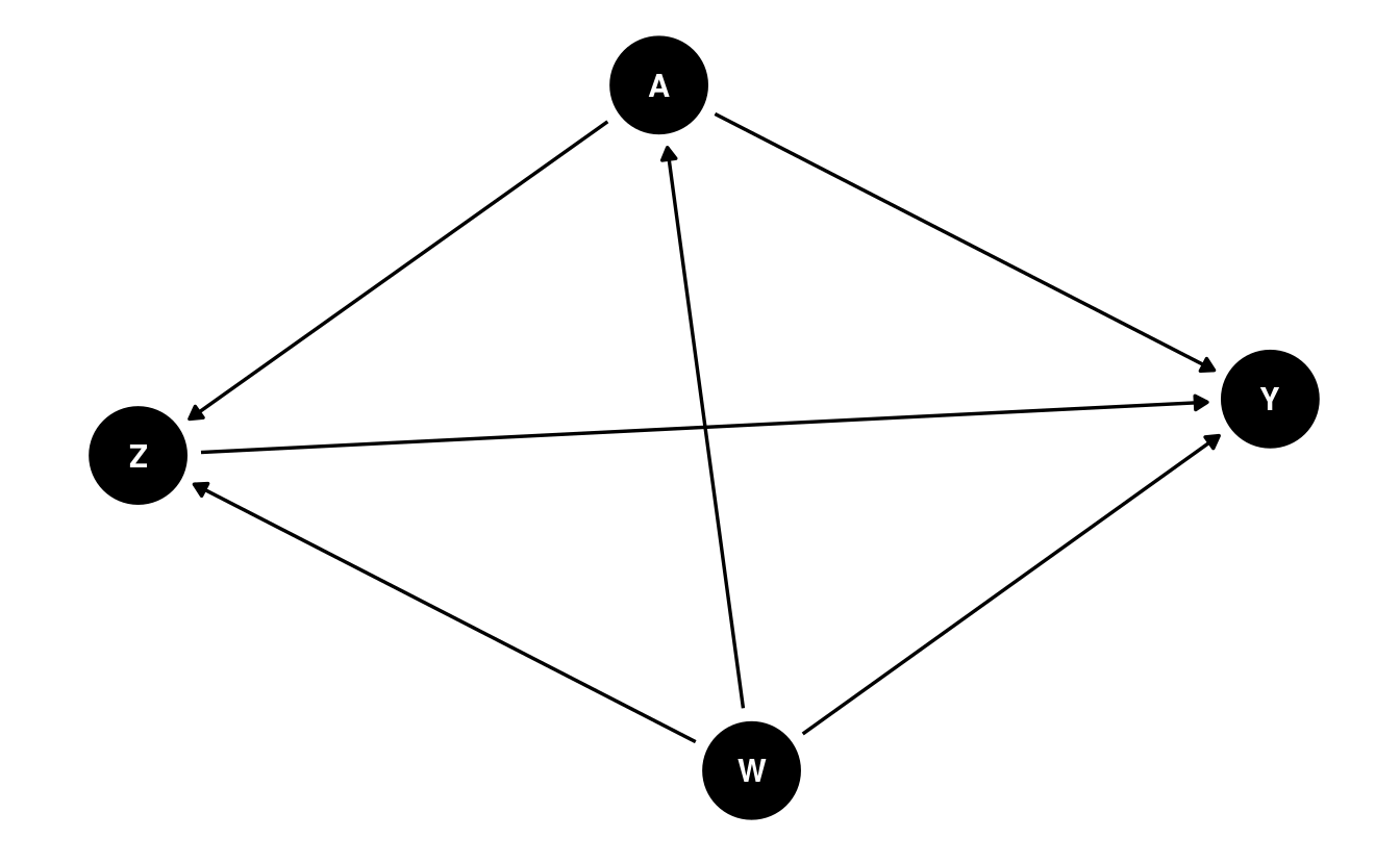
Let us return to our familiar sample of \(n\) units \(O_1, \ldots, O_n\), where we now consider a slightly more complex data structure \(O = (W, A, Z, Y)\) for any given observational unit. As before, \(W\) represents a vector of observed covariates, \(A\) a binary or continuous treatment, and \(Y\) a binary or continuous outcome; the new post-treatment variable \(Z\) represents a (possibly multivariate) set of mediators. Avoiding assumptions unsupported by background scientific knowledge, we assume only that \(O \sim P_0 \in \M\), where \(\M\) is the nonparametric statistical model that places no assumptions on the form of the data-generating distribution \(P_0\).

As in preceding chapters, a structural causal model (SCM) (Pearl, 2009) helps to formalize the definition of our counterfactual variables: \[\begin{align} W &= f_W(U_W) \\ \nonumber A &= f_A(W, U_A) \\ \nonumber Z &= f_Z(W, A, U_Z) \\ \nonumber Y &= f_Y(W, A, Z, U_Y). \tag{10.1} \end{align}\] This set of equations constitutes a mechanistic model generating the observed data \(O\); furthermore, the SCM encodes several fundamental assumptions. Firstly, there is an implicit temporal ordering: \(W\) occurs first, depending only on exogenous factors \(U_W\); \(A\) happens next, based on both \(W\) and exogenous factors \(U_A\); then come the mediators \(Z\), which depend on \(A\), \(W\), and another set of exogenous factors \(U_Z\); and finally appears the outcome \(Y\). We assume neither access to the set of exogenous factors \(\{U_W, U_A, U_Z, U_Y\}\) nor knowledge of the forms of the deterministic generating functions \(\{f_W, f_A, f_Z, f_Y\}\). In practice, any available knowledge about the data-generating experiment should be incorporated into this model – for example, if the data from a randomized controlled trial (RCT), the form of \(f_A\) may be known. The SCM corresponds to the following DAG:

By factorizing the likelihood of the data \(O\), we can express \(p_0\), the density of \(O\) with respect to the product measure, when evaluated on a particular observation \(o\), in terms of several orthogonal components: \[\begin{align} p_0(o) = &q_{0,Y}(y \mid Z = z, A = a, W = w) \\ \nonumber &q_{0,Z}(z \mid A = a, W = w) \\ \nonumber &g_{0,A}(a \mid W = w) \\ \nonumber &q_{0,W}(w).\\ \nonumber \tag{10.2} \end{align}\] In Equation (10.2), \(q_{0, Y}\) is the conditional density of \(Y\) given \(\{Z, A, W\}\), \(q_{0, Z}\) is the conditional density of \(Z\) given \(\{A, W\}\), \(g_{0, A}\) is the conditional density of \(A\) given \(W\), and \(q_{0, W}\) is the marginal density of \(W\). For convenience and consistency of notation, we will define \(\overline{Q}_Y(Z, A, W) := \E[Y \mid Z, A, W]\) and \(g(A \mid W) := \P(A \mid W)\) (i.e., the propensity score).

We have explicitly excluded potential confounders of the mediator-outcome relationship affected by exposure (i.e., variables affected by \(A\) and affecting both \(Z\) and \(Y\)). Mediation analysis in the presence of such variables is challenging (Avin et al., 2005); thus, most efforts to develop definitions of causal direct and indirect effects explicitly assume the absence of such confounders. Without further assumptions, common mediation parameters (the natural direct and indirect effects) cannot be identified in the presence of such confounding, though Tchetgen Tchetgen and VanderWeele (2014) discuss a monotonicity assumption that may be useful when justified by available scientific knowledge about the system under study. The interested reader may wish to consult recent advances in the vast and quickly growing literature on causal mediation analysis, including interventional direct and indirect effects (Didelez et al., 2006; Lok, 2016; Nguyen et al., 2019; Rudolph et al., 2017; VanderWeele et al., 2014; Vansteelandt and Daniel, 2017), whose identification is robust to this complex form of post-treatment confounding. Within this thread of the literature, Dı́az et al. (2020) and Benkeser and Ran (2021) provide considerations of nonparametric effect decompositions and efficiency theory, while Hejazi, Rudolph, et al. (2022) formulate a novel class of effects utilizing stochastic interventions.

10.3 Defining the Natural Direct and Indirect Effects

10.3.1 Decomposing the Average Treatment Effect

The natural direct and indirect effects arise from a decomposition of the ATE: \[\begin{align*} \E[Y(1) - Y(0)] = &\underbrace{\E[Y(1, Z(0)) - Y(0, Z(0))]}_{\text{NDE}} \\ &+ \underbrace{\E[Y(1, Z(1)) - Y(1, Z(0))]}_{\text{NIE}}. \end{align*}\] In particular, the natural indirect effect (NIE) measures the effect of the treatment \(A \in \{0, 1\}\) on the outcome \(Y\) through the mediators \(Z\), while the natural direct effect (NDE) measures the effect of the treatment on the outcome through all other pathways. Identification of the natural direct and indirect effects requires the following non-testable causal assumptions. Note that the standard assumptions of consistency and no interference (i.e., SUTVA (Rubin, 1978, 1980)) hold owing to the fact that (1) the SCM we consider is restricted so as to give rise only to independent and identically distributed (iid) units; and (2) consistency is an implied property of the SCM, as counterfactuals are derived quantities (as opposed to primitive quantities in the potential outcomes framework); Pearl (2010) provides an illuminating discussion on this latter point.

Definition 10.1 (Exchangeability) \(Y(a, z) \indep (A, Z) \mid W\), which further implies that \(\E\{Y(a, z) \mid A=a, W=w, Z=z\} \equiv \E\{Y(a, z) \mid W=w\}\). This is a special, more restrictive case of the standard assumption of no unmeasured counfounding in the presence of mediators. The analogous randomization assumption is simply the standard randomization assumption applied to a joint intervention on both the treatment \(A\) and mediators \(Z\).

Definition 10.2 (Treatment Positivity) For any \(a \in \mathcal{A}\) and \(w \in \mathcal{W}\), the conditional probability of treatment \(g(a \mid w)\) is bounded away from the limits of the unit interval by a small factor \(\xi > 0\). More precisely, \(\xi < g(a \mid w) < 1 - \xi\). This mirrors the standard positivity assumption required for static interventions, discussed previously.

Definition 10.3 (Mediator Positivity) For any \(z \in \mathcal{Z}\), \(a \in \mathcal{A}\), and \(w \in \mathcal{W}\), the conditional mediator density must be bounded away from zero by a small factor \(\epsilon > 0\), specifically, \(\epsilon < q_{0,Z}(z \mid a, w)\). Essentially, this requires that the conditional mediator density be bounded away from zero for all \(\{z, a, w\}\) in their joint support \(\mathcal{Z} \times \mathcal{A} \times \mathcal{W}\), which is to say that it must be possible to observe any given mediator value across all strata defined by both treatment \(A\) and baseline covariates \(W\). A less restrictive form of this assumption is also possible – specifically, that the ratio of the mediator densities under both treatment contrasts be bounded for the two realizations of the mediator density under differing treatment contrasts.

Definition 10.4 (Cross-world Counterfactual Independence) For all \(a \neq a'\), where \(a, a' \in \mathcal{A}\), and \(z \in \mathcal{Z}\), \(Y(a', z)\) must be independent of \(Z(a)\), given \(W\). That is, the counterfactual outcome under the treatment contrast \(a' \in \mathcal{A}\) and the counterfactual mediator value \(Z(a) \in \mathcal{Z}\) (under the alternative contrast \(a \in \mathcal{A}\)) must both be observable. The term “cross-world” refers to the two counterfactuals \(Z(a)\) and \(Y(a', z)\) existing under two differing treatment contrasts. Though their joint distribution is well-defined, these counterfactuals can never be jointly realized.

While the first three assumptions may be familiar based on their analogs in simpler settings, the cross-world independence requirement is unique to identification of the natural direct and indirect effects. This assumption resolves a challenging complication to the identification of these path-specific effects, which has been termed the “recanting witness” by Avin et al. (2005), who introduce a graphical resolution equivalent to this assumption. This independence of counterfactuals indexed by distinct interventions is, in fact, a serious limitation to the scientific relevance of these effect definitions, as it results in the NDE and NIE being unidentifiable in randomized trials (Robins and Richardson, 2010), implying that corresponding scientific claims cannot be falsified through experimentation (Dawid, 2000; Popper, 1934) and, consequently, directly contradicting a foundational pillar of the scientific method.

While many attempts have been made to weaken this last assumption (Imai et al., 2010; Petersen et al., 2006; Vansteelandt et al., 2012; Vansteelandt and VanderWeele, 2012), these results either impose stringent modeling assumptions, propose alternative interpretations of the natural effects, or provide a limited degree of additional flexibility by developing conditions that may more easily be satisfied. For example, Petersen et al. (2006) weaken this assumption by requiring it only for conditional means (rather than distinct counterfactuals) and adopt a view of the natural direct effect as a weighted average of another type of direct effect, the controlled direct effect. The motivated reader may wish to further examine these details independently. We next review estimation of the NDE and NIE, which remain widely used in modern applications of causal mediation analysis.

10.3.2 Estimating the Natural Direct Effect

The NDE is defined as \[\begin{align*} \psi_{\text{NDE}} =&~\E[Y(1, Z(0)) - Y(0, Z(0))] \\ =& \sum_w \sum_z [\underbrace{\E(Y \mid A = 1, z, w)}_{\overline{Q}_Y(A = 1, z, w)} - \underbrace{\E(Y \mid A = 0, z, w)}_{\overline{Q}_Y(A = 0, z, w)}] \\ &\times \underbrace{p(z \mid A = 0, w)}_{q_Z(Z \mid 0, w))} \underbrace{p(w)}_{q_W}, \end{align*}\] where the likelihood factors arise from a factorization of the joint likelihood: \[\begin{equation*} p(w, a, z, y) = \underbrace{p(y \mid w, a, z)}_{q_Y(A, W, Z)} \underbrace{p(z \mid w, a)}_{q_Z(Z \mid A, W)} \underbrace{p(a \mid w)}_{g(A \mid W)} \underbrace{p(w)}_{q_W}. \end{equation*}\]

The process of estimating the NDE begins by constructing \(\overline{Q}_{Y, n}\), an estimate of the conditional mean of the outcome, given \(Z\), \(A\), and \(W\). With an estimate of this conditional mean in hand, predictions of the quantities \(\overline{Q}_Y(Z, 1, W)\) (setting \(A = 1\)) and, likewise, \(\overline{Q}_Y(Z, 0, W)\) (setting \(A = 0\)) are readily obtained. We denote the difference of these conditional means \(\overline{Q}_{\text{diff}} = \overline{Q}_Y(Z, 1, W) - \overline{Q}_Y(Z, 0, W)\), which is itself only a functional parameter of the data distribution. \(\overline{Q}_{\text{diff}}\) captures differences in the conditional mean of \(Y\) across contrasts of \(A\).

A procedure for constructing a targeted maximum likelihood (TML) estimator of the NDE treats \(\overline{Q}_{\text{diff}}\) itself as a nuisance parameter, regressing its estimate \(\overline{Q}_{\text{diff}, n}\) on baseline covariates \(W\), among observations in the control condition only (i.e., those for whom \(A = 0\) is observed); the goal of this step is to remove part of the marginal impact of \(Z\) on \(\overline{Q}_{\text{diff}}\), since the covariates \(W\) precede the mediators \(Z\) in time. Regressing this difference on \(W\) among the controls recovers the expected \(\overline{Q}_{\text{diff}}\), under the setting in which all individuals are treated as falling in the control condition \(A = 0\). Any residual additive effect of \(Z\) on \(\overline{Q}_{\text{diff}}\) is removed during the TML estimation step using the auxiliary (or “clever”) covariate, which accounts for the mediators \(Z\). This auxiliary covariate takes the form

\[\begin{equation*} C_Y(q_Z, g)(O) = \Bigg\{\frac{\mathbb{I}(A = 1)}{g(1 \mid W)} \frac{q_Z(Z \mid 0, W)}{q_Z(Z \mid 1, W)} - \frac{\mathbb{I}(A = 0)}{g(0 \mid W)} \Bigg\} \ . \end{equation*}\] Breaking this down, \(\mathbb{I}(A = 1) / g(1 \mid W)\) is the inverse propensity score weight for \(A = 1\) and, likewise, \(\mathbb{I}(A = 0) / g(0 \mid W)\) is the inverse propensity score weight for \(A = 0\). The middle term is the ratio of the conditional densities of the mediator under the control (\(A = 0\)) and treatment (\(A = 1\)) conditions (n.b., recall the mediator positivity condition above).

This subtle appearance of a ratio of conditional densities is concerning – tools to estimate such quantities are sparse in the statistics literature (Dı́az and van der Laan, 2011; Hejazi, Benkeser, et al., 2022), unfortunately, and the problem is still more complicated (and computationally taxing) when \(Z\) is high-dimensional. As only the ratio of these conditional densities is required, a convenient re-parametrization may be achieved, that is, \[\begin{equation*} \frac{p(A = 0 \mid Z, W)}{g(0 \mid W)} \frac{g(1 \mid W)}{p(A = 1 \mid Z, W)} \ . \end{equation*}\] Going forward, we will denote this re-parameterized conditional probability functional \(e(A \mid Z, W) := p(A \mid Z, W)\). The same re-parameterization technique has been used by Zheng and van der Laan (2012), Tchetgen Tchetgen (2013), Dı́az and Hejazi (2020), Dı́az et al. (2020), and Hejazi, Rudolph, et al. (2022) in similar contexts. This reformulation is particularly useful for the fact that it reduces the estimation problem to one requiring only the estimation of conditional means, opening the door to the use of a wide range of machine learning algorithms, as discussed previously.

Underneath the hood, the mean outcome difference \(\overline{Q}_{\text{diff}}\) and \(e(A \mid Z, W)\), the conditional probability of \(A\) given \(Z\) and \(W\), are used in constructing the auxiliary covariate for TML estimation. These nuisance parameters play an important role in the bias-correcting update step of the TML estimation procedure.

10.3.3 Estimating the Natural Indirect Effect

Derivation and estimation of the NIE is analogous to that of the NDE. Recall that the NIE is the effect of \(A\) on \(Y\) only through the mediator \(Z\). This counterfactual quantity, which may be expressed \(\E(Y(Z(1), 1) - \E(Y(Z(0), 1)\), corresponds to the difference of the conditional mean of \(Y\) given \(A = 1\) and \(Z(1)\) (the values the mediator would take under \(A = 1\)) and the conditional expectation of \(Y\) given \(A = 1\) and \(Z(0)\) (the values the mediator would take under \(A = 0\)).

As with the NDE, re-parameterization can be used to replace \(q_Z(Z \mid A, W)\) with \(e(A \mid Z, W)\) in the estimation process, avoiding estimation of a possibly multivariate conditional density. However, in this case, the mediated mean outcome difference, previously computed by regressing \(\overline{Q}_{\text{diff}}\) on \(W\) among the control units (for whom \(A = 0\) is observed) is instead replaced by a two-step process. First, \(\overline{Q}_Y(Z, 1, W)\), the conditional mean of \(Y\) given \(Z\) and \(W\) when \(A = 1\), is regressed on \(W\), among only the treated units (i.e., for whom \(A = 1\) is observed). Then, the same quantity, \(\overline{Q}_Y(Z, 1, W)\) is again regressed on \(W\), but this time among only the control units (i.e., for whom \(A = 0\) is observed). The mean difference of these two functionals of the data distribution is a valid estimator of the NIE. It can be thought of as the additive marginal effect of treatment on the conditional mean of \(Y\) given \((W, A = 1, Z)\) through its effect on \(Z\). So, in the case of the NIE, while our estimand \(\psi_{\text{NIE}}\) is different, the same estimation techniques useful for constructing efficient estimators of the NDE come into play.

10.4 The Population Intervention Direct and Indirect Effects

At times, the natural direct and indirect effects may prove too limiting, as these effect definitions are based on static interventions (i.e., setting \(A = 0\) or \(A = 1\)), which may be unrealistic for real-world interventions. In such cases, one may turn instead to the population intervention direct effect (PIDE) and the population intervention indirect effect (PIIE), which are based on decomposing the effect of the population intervention effect (PIE) of flexible stochastic interventions (Dı́az and Hejazi, 2020).

We previously discussed stochastic interventions when considering how to intervene on continuous-valued treatments; however, these intervention schemes may be applied to all manner of treatment variables. A particular type of stochastic intervention well-suited to working with binary treatments is the incremental propensity score intervention (IPSI), first proposed by Kennedy (2019). Such interventions do not deterministically set the treatment level of an observed unit to a fixed quantity (i.e., setting \(A = 1\)), but instead alter the odds of receiving the treatment by a fixed amount (\(0 \leq \delta \leq \infty\)) for each individual. In particular, this intervention takes the form \[\begin{equation*} g_{\delta}(1 \mid w) = \frac{\delta g(1 \mid w)}{\delta g(1 \mid w) + 1 - g(1\mid w)}, \end{equation*}\] where the scalar \(0 < \delta < \infty\) specifies a change in the odds of receiving treatment. As described by Dı́az and Hejazi (2020) in the context of causal mediation analysis, the identification assumptions required for the PIDE and the PIIE are significantly more lax than those required for the NDE and NIE. These identification assumptions include the following. Importantly, the assumption of cross-world counterfactual independence is not at all required.

Definition 10.5 (Conditional Exchangeability of Treatment and Mediators) Assume that \(\E\{Y(a, z) \mid Z, A, W\} = \E\{Y(a, z) \mid Z, W\}~\forall~(a, z) \in \mathcal{A} \times \mathcal{Z}W\). This assumption is stronger than and implied by the assumption \(Y(a, z) \indep (A,Z) \mid W\), originally proposed by Vansteelandt and VanderWeele (2012) for identification of mediated effects among the treated. In introducing this assumption Dı́az and Hejazi (2020) state that “This assumption would be satisfied for any pre-exposure \(W\) in a randomized experiment in which exposure and mediators are randomized. Thus, the direct effect for a population intervention corresponds to contrasts between treatment regimes of a randomized experiment via interventions on \(A\) and \(Z\), unlike the natural direct effect for the average treatment effect (Robins and Richardson, 2010).”

Definition 10.6 (Common Support of Treatment and Mediators) Assume that \(\text{supp}\{g_{\delta}(\cdot \mid w)\} \subseteq \text{supp}\{g(\cdot \mid w)\}~\forall~w \in \mathcal{W}\). This assumption is standard and requires only that the post-intervention value of \(A\) be supported in the data. Note that this is significantly weaker than the treatment and mediator positivity conditions required for the natural direct and indirect effects, and it is a direct consequence of using stochastic (rather than static) interventions.

10.4.1 Decomposing the Population Intervention Effect

We may decompose the population intervention effect (PIE) in terms of the population intervention direct effect (PIDE) and the population intervention indirect effect (PIIE): \[\begin{equation*} \mathbb{E}\{Y(A_\delta)\} - \mathbb{E}Y = \overbrace{\mathbb{E}\{Y(A_\delta, Z(A_\delta)) - Y(A_\delta, Z)\}}^{\text{PIIE}} + \overbrace{\mathbb{E}\{Y(A_\delta, Z) - Y(A, Z)\}}^{\text{PIDE}}. \end{equation*}\]

This decomposition of the PIE as the sum of the population intervention direct and indirect effects has an interpretation analogous to the corresponding standard decomposition of the average treatment effect. In the sequel, we will compute each of the components of the direct and indirect effects above using appropriate estimators as follows

• For \(\E\{Y(A, Z)\}\), the sample mean \(\frac{1}{n}\sum_{i=1}^n Y_i\) is consistent;
• for \(\E\{Y(A_{\delta}, Z)\}\), a TML estimator for the effect of a joint intervention altering the treatment mechanism but not the mediation mechanism, based on the proposal in Dı́az and Hejazi (2020); and,
• for \(\E\{Y(A_{\delta}, Z_{A_{\delta}})\}\), an efficient estimator for the effect of a joint intervention on both the treatment and mediation mechanisms, as per Kennedy (2019).

10.4.2 Estimating the Effect Decomposition Term

As described by Dı́az and Hejazi (2020), the statistical functional identifying the decomposition term that appears in both the PIDE and PIIE \(\E\{Y(A_{\delta}, Z)\}\), which corresponds to altering the treatment mechanism while keeping the mediation mechanism fixed, is \[\begin{equation*} \psi_0(\delta) = \int \overline{Q}_{0,Y}(a, z, w) g_{0,\delta}(a \mid w) p_0(z, w) d\nu(a, z, w), \end{equation*}\] for which a TML estimator is available. In the case of \(A \in \{0, 1\}\), the efficient influence function (EIF) with respect to the nonparametric statistical model \(\mathcal{M}\) is \(D_{\delta}(o) = D^Y_{\delta}(o) + D^A_{\delta}(o) + D^{Z,W}_{\delta}(o) - \psi(\delta)\), where the orthogonal components of the EIF are defined as follows:

• \(D^Y_{\delta}(o) = \{g_{\delta}(a \mid w) / e(a \mid z, w)\} \{y - \overline{Q}_{Y}(z,a,w)\}\),
• \(D^A_{\delta}(o) = \{\delta\phi(w) (a - g(1 \mid w))\} / \{(\delta g(1 \mid w) + g(0 \mid w))^2\}\), and where \(\phi(w) := \E\{\overline{Q}_{Y}(1, Z, W) - \overline{Q}_{Y}(0, Z, W) \mid W = w\}\),
• \(D^{Z,W}_{\delta}(o) = \int_{\mathcal{A}} \overline{Q}_{Y}(z, a, w) g_{\delta}(a \mid w) d\kappa(a)\).

The TML estimator may be computed by fluctuating initial estimates of the nuisance parameters so as to solve the EIF estimating equation. The resultant TML estimator is \[\begin{equation*} \psi_{n}^{\star}(\delta) = \int_{\mathcal{A}} \frac{1}{n} \sum_{i=1}^n \overline{Q}_{Y,n}^{\star}(Z_i, a, W_i) g_{\delta, n}^{\star}(a \mid W_i) d\kappa(a), \end{equation*}\] where \(g_{\delta,n}^{\star}(a \mid w)\) and \(\overline{Q}_{Y,n}^{\star}(z,a,w)\) are generated by regressions that fluctuate (or tilt) initial nuisance parameter estimates towards solutions of the score equations \(n^{-1} \sum_{i=1}^n D^A_{\delta}(O_i) = 0\) and \(n^{-1} \sum_{i=1}^n D^Y_{\delta}(O_i) = 0\), respectively. This TML estimator \(\psi_{n}^{\star}(\delta)\) is implemented in tmle3mediate package. We demonstrate the use of tmle3mediate to obtain \(\E\{Y(A_{\delta}, Z)\}\) via its TML estimator in the following worked code examples.

10.5 Evaluating the Direct and Indirect Effects

We now turn to estimating the natural direct and indirect effects, as well as the population intervention direct effect, using the WASH Benefits data, introduced in earlier chapters. Let’s first load the data:

library(data.table)
library(sl3)
library(tmle3)
library(tmle3mediate)

# download data
washb_data <- fread(
  paste0(
    "https://raw.githubusercontent.com/tlverse/tlverse-data/master/",
    "wash-benefits/washb_data.csv"
  ),
  stringsAsFactors = TRUE
)

# make intervention node binary and subsample
washb_data <- washb_data[sample(.N, 600), ]
washb_data[, tr := as.numeric(tr != "Control")]

We’ll next define the baseline covariates \(W\), treatment \(A\), mediators \(Z\), and outcome \(Y\) nodes of the NPSEM via a “Node List” object:

node_list <- list(
  W = c(
    "momage", "momedu", "momheight", "hfiacat", "Nlt18", "Ncomp", "watmin",
    "elec", "floor", "walls", "roof"
  ),
  A = "tr",
  Z = c("sex", "month", "aged"),
  Y = "whz"
)

Here, the node_list encodes the parents of each node – for example, \(Z\) (the mediators) have parents \(A\) (the treatment) and \(W\) (the baseline confounders), and \(Y\) (the outcome) has parents \(Z\), \(A\), and \(W\). We’ll also handle any missingness in the data by invoking process_missing:

processed <- process_missing(washb_data, node_list)
washb_data <- processed$data
node_list <- processed$node_list

We’ll now construct an ensemble learner using a handful of popular machine learning algorithms:

# SL learners used for continuous data (the nuisance parameter Z)
enet_contin_learner <- Lrnr_glmnet$new(
  alpha = 0.5, family = "gaussian", nfolds = 3
)
lasso_contin_learner <- Lrnr_glmnet$new(
  alpha = 1, family = "gaussian", nfolds = 3
)
fglm_contin_learner <- Lrnr_glm_fast$new(family = gaussian())
mean_learner <- Lrnr_mean$new()
contin_learner_lib <- Stack$new(
  enet_contin_learner, lasso_contin_learner, fglm_contin_learner, mean_learner
)
sl_contin_learner <- Lrnr_sl$new(learners = contin_learner_lib)

# SL learners used for binary data (nuisance parameters G and E in this case)
enet_binary_learner <- Lrnr_glmnet$new(
  alpha = 0.5, family = "binomial", nfolds = 3
)
lasso_binary_learner <- Lrnr_glmnet$new(
  alpha = 1, family = "binomial", nfolds = 3
)
fglm_binary_learner <- Lrnr_glm_fast$new(family = binomial())
binary_learner_lib <- Stack$new(
  enet_binary_learner, lasso_binary_learner, fglm_binary_learner, mean_learner
)
sl_binary_learner <- Lrnr_sl$new(learners = binary_learner_lib)

# create list for treatment and outcome mechanism regressions
learner_list <- list(
  Y = sl_contin_learner,
  A = sl_binary_learner
)

10.5.1 Targeted Estimation of the Natural Indirect Effect

We demonstrate calculation of the NIE below, starting by instantiating a “Spec” object that encodes exactly which learners to use for the nuisance parameters \(e(A \mid Z, W)\) and \(\psi_Z\). We then pass our Spec object to the tmle3 function, alongside the data, the node list (created above), and a learner list indicating which machine learning algorithms to use for estimating the nuisance parameters based on \(A\) and \(Y\).

tmle_spec_NIE <- tmle_NIE(
  e_learners = Lrnr_cv$new(lasso_binary_learner, full_fit = TRUE),
  psi_Z_learners = Lrnr_cv$new(lasso_contin_learner, full_fit = TRUE),
  max_iter = 1
)
washb_NIE <- tmle3(
  tmle_spec_NIE, washb_data, node_list, learner_list
)
washb_NIE
A tmle3_Fit that took 1 step(s)
   type                  param init_est tmle_est      se    lower   upper
1:  NIE NIE[Y_{A=1} - Y_{A=0}] 0.002419 0.003376 0.04342 -0.08173 0.08848
   psi_transformed lower_transformed upper_transformed
1:        0.003376          -0.08173           0.08848

Based on the output, we conclude that the indirect effect of the treatment through the mediators (sex, month, aged) is 0.0034.

10.5.2 Targeted Estimation of the Natural Direct Effect

An analogous procedure applies for estimation of the NDE, only replacing the Spec object for the NIE with tmle_spec_NDE to define learners for the NDE nuisance parameters:

tmle_spec_NDE <- tmle_NDE(
  e_learners = Lrnr_cv$new(lasso_binary_learner, full_fit = TRUE),
  psi_Z_learners = Lrnr_cv$new(lasso_contin_learner, full_fit = TRUE),
  max_iter = 1
)
washb_NDE <- tmle3(
  tmle_spec_NDE, washb_data, node_list, learner_list
)
washb_NDE
A tmle3_Fit that took 1 step(s)
   type                  param init_est tmle_est      se   lower  upper
1:  NDE NDE[Y_{A=1} - Y_{A=0}]  0.01551  0.01551 0.08579 -0.1526 0.1837
   psi_transformed lower_transformed upper_transformed
1:         0.01551           -0.1526            0.1837

From this, we can draw the conclusion that the direct effect of the treatment (through all paths not involving the mediators (sex, month, aged)) is 0.0155. Note that, together, the estimates of the natural direct and indirect effects approximately recover the average treatment effect, that is, based on these estimates of the NDE and NIE, the ATE is roughly 0.0189.

10.5.3 Targeted Estimation of the Population Intervention Direct Effect

As previously noted, the assumptions underlying the natural direct and indirect effects may be challenging to justify; moreover, the effect definitions themselves depend on the application of a static intervention to the treatment, sharply limiting their flexibility. When considering binary treatments, incremental propensity score shifts provide an alternative class of flexible, stochastic interventions. We’ll now consider estimating the PIDE with an IPSI that modulates the odds of receiving treatment by \(\delta = 3\). Such an intervention may be interpreted (hypothetically) as the effect of a design that encourages study participants to opt in to receiving the treatment, thus increasing their relative odds of receiving said treatment. To exemplify our approach, we postulate a motivational intervention that triples the odds (i.e., \(\delta = 3\)) of receiving the treatment for each individual:

# set the IPSI multiplicative shift
delta_ipsi <- 3

# instantiate tmle3 spec for stochastic mediation
tmle_spec_pie_decomp <- tmle_medshift(
  delta = delta_ipsi,
  e_learners = Lrnr_cv$new(lasso_binary_learner, full_fit = TRUE),
  phi_learners = Lrnr_cv$new(lasso_contin_learner, full_fit = TRUE)
)

# compute the TML estimate
washb_pie_decomp <- tmle3(
  tmle_spec_pie_decomp, washb_data, node_list, learner_list
)
washb_pie_decomp

# get the PIDE
washb_pie_decomp$summary$tmle_est - mean(washb_data[, get(node_list$Y)])

Recall that, based on the decomposition outlined previously, the PIDE may be denoted \(\beta_{0,\text{PIDE}}(\delta) = \psi_0(\delta) - \E Y\). Thus, a TML estimator of the PIDE, \(\beta_{n,\text{PIDE}}(\delta)\) may be expressed as a composition of estimators of its constituent parameters: \[\begin{equation*} \beta_{n,\text{PIDE}}({\delta}) = \psi^{\star}_{n}(\delta) - \frac{1}{n} \sum_{i = 1}^n Y_i. \end{equation*}\]

10.6 Exercises

10.6.1 Review of Key Concepts

Exercise 10.1 Examine the WASH Benefits dataset and choose a different set of potential mediators of the effect of the treatment on weight-for-height Z-score. Using this newly chosen set of mediators (or single mediator), estimate the natural direct and indirect effects. Provide an interpretation of these estimates.

Solution. Forthcoming

Exercise 10.2 Assess whether additivity of the natural direct and indirect effects holds. Using the natural direct and indirect effects estimated above, does their sum recover the ATE?

Solution. Forthcoming

Exercise 10.3 Evaluate whether the assumptions required for identification of the natural direct and indirect effects are plausible in the WASH Benefits example. In particular, position this evaluation in terms of empirical diagnostics of treatment and mediator positivity.

Solution. Forthcoming

10.6.2 The Ideas in Action

Exercise 10.4 Forthcoming

Solution. Forthcoming

Exercise 10.5 Forthcoming

Solution. Forthcoming