5 Cross-validation
Ivana Malenica
Based on the origami R package
by Jeremy Coyle, Nima Hejazi, Ivana Malenica and Rachael Phillips.
Learning Objectives
By the end of this chapter you will be able to:
Differentiate between training, validation and test sets.
Understand the concept of a loss function, risk and cross-validation.
Select a loss function that is appropriate for the functional parameter to be estimated.
Understand and contrast different cross-validation schemes for i.i.d. data.
Understand and contrast different cross-validation schemes for time dependent data.
Setup the proper fold structure, build custom fold-based function, and cross-validate the proposed function using the
origamiRpackage.Setup the proper cross-validation structure for the use by the Super Learner using the the
origamiRpackage.
5.1 Introduction
Following the Roadmap for Targeted Learning, we start to elaborate
on the estimation step in the current chapter. In order to generate an estimate
of the target parameter, we need to decide how to evaluate the quality of our
estimation procedure’s performance. The performance, or error, of any algorithm
(estimator) corresponds to its generalizability to independent datasets arising
from the same data-generating process. Assessment of the performance of an
algorithm is extremely important — it provides a quantitative measure of how
well the algorithm performs, and it guides the choice of selecting among a set
(or “library”) of algorithms. In order to assess the performance of an
algorithm, or a library of them, we introduce the concept of a loss
function, which defines the risk or the expected prediction error.
Our goal is to estimate the true performance (risk) of our estimator. In the
next chapter, we elaborate on how to estimate the performance of a library of
algorithms in order to choose the best-performing one. In the following, we
propose a method to do so using the observed data and cross-validation
procedures implemented in the origami package (Coyle et al., n.d.; Coyle and Hejazi, 2018).
5.2 Background
Ideally, in a data-rich scenario (i.e., one with unlimited observations), we would split our dataset into three parts:
- the training set,
- the validation set, and
- the test (or holdout) set.
The training set is used to fit algorithm(s) of interest; we evaluate the performance of the fit(s) on a validation set, which can be used to estimate prediction error (e.g., for algorithm tuning or selection). The final error of the selected algorithm is obtained by using the test (or holdout) set, which is kept entirely separate such that the algorithms never encounter these observations until the final model evaluation step. One might wonder, with training data readily available, why not use the training error to evaluate the proposed algorithm’s performance? Unfortunately, the training error is a biased estimate of a fitted algorithm’s generalizability, since it uses the same data for fitting and evaluation.
Since data are often scarce, separating a dataset into training, validation and test sets can prove too limiting, on account of decreasing the available data for use in training by too much. In the absence of a large dataset and a designated test set, we must resort to methods that estimate the algorithm’s true performance by efficient sample re-use. Re-sampling methods, like the bootstrap, involve repeatedly sampling from the training set and fitting the algorithms to these samples. While often computationally intensive, re-sampling methods are particularly useful for evaluating an algorithm and selecting among a set of them. In addition, they provide more insight on the variability and robustness of a fitted algorithm, relative to fitting an algorithm only once to all of the training data.
5.2.1 Introducing: cross-validation
In this chapter, we focus on cross-validation — an essential tool for evaluating how any algorithm extends from a sample of data to the target population from which it arose. Cross-validation has seen widespread application in all facets of modern statistics, and perhaps most notably in statistical machine learning. The cross-validation procedure has been proven to be optimal for algorithm selection in large samples, i.e. asymptotically. In particular,cross-validated algorithm estimates the true risk when the estimate is applied to an independent sample from the joint distribution of the predictors and outcome.
When used for model selection, cross-validation has powerful optimality properties. The asymptotic optimality results state that the cross-validated selector performs (in terms of risk) asymptotically as well as an optimal oracle selector — a hypothetical procedure with free access to the true, unknown data-generating distribution. For further details on the theoretical results, we suggest consulting van der Laan and Dudoit (2003), van der Laan et al. (2004), Dudoit and van der Laan (2005) and van der Vaart et al. (2006).
The origami package provides a suite of tools for cross-validation. In the
following, we describe different types of cross-validation schemes readily
available in origami, introduce the general structure of the origami
package, and demonstrate the use of these procedures in various applied
settings.
5.3 Estimation Roadmap: How does it all fit together?
Similarly to how we defined the Roadmap for Targeted Learning, we can define the Estimation Roadmap as a guide for the estimation process. In particular, the unified loss-based estimation framework (Dudoit and van der Laan, 2005; van der Laan et al., 2004, 2007; van der Laan and Dudoit, 2003; van der Vaart et al., 2006), which relies on cross-validation for estimator construction, selection, and performance assessment, consists of three main steps:
Loss function: Define the target parameter as the minimizer of the expected loss (risk) for a full data loss function chosen to represent the desired performance measure. By full data, we refer to the complete data including missingness process, for example. Map the full data loss function into an observed data loss function, having the same expected value and leading to an estimator of risk.
Algorithms: Construct a finite collection of candidate estimators of the parameter of interest.
Cross-validation scheme: Apply appropriate cross-validation, and use the cross-validated risk in order to select the best performing estimator among the candidates. Assess the overall performance of the resulting estimator.
5.4 Example: Cross-validation and Prediction
Having introduced the Estimation Roadmap, we can more precisely define our objective using prediction as an example. Let the observed data be defined as \(O = (W, Y)\), where a unit specific data structure can be written as \(O_i = (W_i, Y_i)\), for \(i = 1, \ldots, n\). We denote \(Y_i\) as the outcome/dependent variable of interest, and \(W_i\) as a \(p\)-dimensional set of covariate (predictor) variables. We assume the \(n\) units are independent, or conditionally independent, and identically distributed. Let \(\psi_0(W)\) denote the target parameter of interest, the quantity we wish to estimate (estimand). For this example, we are interested in estimating the conditional expectation of the outcome given the covariates, \(\psi_0(W) = \E(Y \mid W)\). Following the Estimation Roadmap, we choose the appropriate loss function, \(L\), such that \(\psi_0(W) = \text{argmin}_{\psi} \E_0[L(O, \psi(W))]\). Note that \(\psi_0(W)\), the true target parameter, is a minimizer of the risk (expected value of the chosen loss function). The appropriate loss function for conditional expectation with continuous outcome could be a mean squared error, for example. Then we can define \(L\) as \(L(O, \psi(W)) = (Y_i -\psi(W_i)^2\). Note that there can be many different algorithms which estimate the estimand (many different \(\psi\)s). How do we know how well each of the candidate estimators of \(\psi_0(W)\) are doing? To pick the best-performing candidate estimator and assess its overall performance, we use cross-validation. Observations in the training set are used to fit (or train) the estimator, while those in validation set are used to assess the risk of (or validate) it.
Next, we introduce notation flexible enough to represent any cross-validation scheme. In particular, we define a split vector, \(B_n = (B_n(i): i = 1, \ldots, n) \in \{0,1\}^n\). A realization of \(B_n\) defines a random split of the data into training and validation subsets such that if \[B_n(i) = 0, \ \ \text{i sample is in the training set}\] \[B_n(i) = 1, \ \ \text{i sample is in the validation set.}\] We can further define \(P_{n, B_n}^0\) and \(P_{n, B_n}^1\) as the empirical distributions of the training and validation sets, respectively. Then, \(n_0 = \sum_i (1 - B_n(i))\) and \(n_1 = \sum_i B_n(i)\) denote the number of samples in the training and validation sets, respectively. The particular distribution of the split vector \(B_n\) defines the type of cross-validation scheme, tailored to the problem and dataset at hand.
5.5 Cross-validation schemes in origami
A variety of different partitioning schemes exist, each tailored to the salient
details of the problem of interest, including data size, prevalence of the
outcome, and dependence structure (between units or across time). In the
following, we describe different cross-validation schemes available in the
origami package, and we go on to demonstrate their use in practical data
analysis examples.
WASH Benefits Study Example
In order to illustrate different cross-validation schemes, we will be using the
WASH Benefits example dataset (detailed information can be found in
Chapter 3). In particular, we are interested in predicting
weight-for-height Z-score (whz) using the available covariate data. For this
illustration, we will start by treating the data as independent and identically
distributed (i.i.d.) random draws from an unknown distribution \(P_0\). To
see what each cross-validation scheme is doing, we will subset the data to only
\(n=30\). Note that each row represents an i.i.d. sampled unit, indexed by the row
number.
library(data.table)
library(origami)
library(knitr)
library(dplyr)

# load data set and take a peek
washb_data <- fread(
  paste0(
    "https://raw.githubusercontent.com/tlverse/tlverse-data/master/",
    "wash-benefits/washb_data.csv"
  ),
  stringsAsFactors = TRUE
)| whz | tr | fracode | month | aged | sex | momage | momedu | momheight | hfiacat | Nlt18 | Ncomp | watmin | elec | floor | walls | roof | asset_wardrobe | asset_table | asset_chair | asset_khat | asset_chouki | asset_tv | asset_refrig | asset_bike | asset_moto | asset_sewmach | asset_mobile |
|---|---|---|---|---|---|---|---|---|---|---|---|---|---|---|---|---|---|---|---|---|---|---|---|---|---|---|---|
| 0.00 | Control | N05265 | 9 | 268 | male | 30 | Primary (1-5y) | 146.4 | Food Secure | 3 | 11 | 0 | 1 | 0 | 1 | 1 | 0 | 1 | 1 | 1 | 0 | 1 | 0 | 0 | 0 | 0 | 1 |
| -1.16 | Control | N05265 | 9 | 286 | male | 25 | Primary (1-5y) | 148.8 | Moderately Food Insecure | 2 | 4 | 0 | 1 | 0 | 1 | 1 | 0 | 1 | 0 | 1 | 1 | 0 | 0 | 0 | 0 | 0 | 1 |
| -1.05 | Control | N08002 | 9 | 264 | male | 25 | Primary (1-5y) | 152.2 | Food Secure | 1 | 10 | 0 | 0 | 0 | 1 | 1 | 0 | 0 | 1 | 0 | 1 | 0 | 0 | 0 | 0 | 0 | 1 |
| -1.26 | Control | N08002 | 9 | 252 | female | 28 | Primary (1-5y) | 140.2 | Food Secure | 3 | 5 | 0 | 1 | 0 | 1 | 1 | 1 | 1 | 1 | 1 | 0 | 0 | 0 | 1 | 0 | 0 | 1 |
| -0.59 | Control | N06531 | 9 | 336 | female | 19 | Secondary (>5y) | 150.9 | Food Secure | 2 | 7 | 0 | 1 | 0 | 1 | 1 | 1 | 1 | 1 | 1 | 1 | 0 | 0 | 0 | 0 | 0 | 1 |
| -0.51 | Control | N06531 | 9 | 304 | male | 20 | Secondary (>5y) | 154.2 | Severely Food Insecure | 0 | 3 | 1 | 1 | 0 | 1 | 1 | 0 | 0 | 0 | 0 | 1 | 0 | 0 | 0 | 0 | 0 | 1 |
Above is a look at the first 30 of the data.
5.5.1 Cross-validation for i.i.d. data
5.5.1.1 Re-substitution
The re-substitution method is perhaps the simplest strategy for estimating the risk of a fitted algorithm. With this cross-validation scheme, all observed data units are used in both the training and validation set.
We illustrate the usage of the re-substitution method with origami below,
using the function folds_resubstitution. In order to set up
folds_resubstitution, we need only to specify the total number of sampled
units that we want to allocate to the training and validation sets; remember
that each row of the dataset is a unique i.i.d. sampled unit. Also, notice the
structure of the origami output:
- v: the cross-validation fold
- training_set: the indices of the samples in the training set
- validation_set: the indices of the samples in the training set.
The structure of the origami output, a list of fold(s), holds across all of
the cross-validation schemes presented in this chapter. Below, we show the fold
generated by the re-substitution method:
folds <- folds_resubstitution(nrow(washb_data))
folds
[[1]]
$v
[1] 1

$training_set
 [1]  1  2  3  4  5  6  7  8  9 10 11 12 13 14 15 16 17 18 19 20 21 22 23 24 25
[26] 26 27 28 29 30

$validation_set
 [1]  1  2  3  4  5  6  7  8  9 10 11 12 13 14 15 16 17 18 19 20 21 22 23 24 25
[26] 26 27 28 29 30

attr(,"class")
[1] "fold"
5.5.1.2 Holdout
The holdout method, or the validation set approach, consists of randomly dividing the available data into training and validation (holdout) sets. The model is then fitted (i.e., “trained”) using the observations in the training set and subsequently evaluated (i.e., “validated”) using the observations in the validation set. Typically, the dataset is split into \(60:40\), \(70:30\), \(80:20\) or even \(90:10\) training-to-validation splits.
The holdout method is intuitive and computationally inexpensive; however, it does carry a disadvantage: If we were to repeat the process of randomly splitting the data into training and validation sets, we could get very different cross-validated estimates of the empirical risk. In particular, the empirical mean of the loss function (i.e., the empirical risk) evaluated over the validation set(s) could be highly variable, depending on which samples were included in the training and validation splits. Overall, the cross-validated empirical risk for the holdout method is more variable, since in includes variability of the random split as well — this is not desirable. For classification problems (with a binary or categorical outcome variable), there is an additional disadvantage: it is possible for the training and validation sets to end up with uneven distributions of the two (or more) outcome classes, leading to better training and poor validation, or vice-versa — though this may be corrected by incorporating stratification into the cross-validation process. Finally, note that we are not using all of the data in training or in evaluating the performance of the proposed algorithm, which could itself introduce bias.
5.5.1.3 Leave-one-out
The leave-one-out cross-validation scheme is closely related to the holdout method, as it also involves splitting the dataset into training and validation sets; however, instead of partitioning the dataset into sets of similar size, a single observation is used as the validation set. In doing so, the vast majority of the sampled units are employed for fitting (or training) the candidate learning algorithm. Since only a single sampled unit (for example \(O_1 = (W_1, Y_1)\)) is left out of the fitting process, leave-one-out cross-validation can result in a less biased estimate of the risk. Typically, the leave-one-out approach will not overestimate the risk as much as the holdout method does. On the other hand, since the estimate of risk is based on a single sampled unit, it is usually a highly variable estimate.
We can repeat the process of spiting the dataset into training and validation sets until all of the sampled units have had a chance to act as the validation set. Continuing the example above, a subsequent iteration of the leave-one-out cross-validation scheme may use \(O_2 = (W_2, Y_2)\) as the validation set (where, before, \(O_1 = (W_1, Y_1)\) played that role), while the remaining \(n-1\) sampled units are included in the training set. Repeating this approach \(n\) times results in \(n\) risk estimates, for example, \(MSE_1, MSE_2, \ldots, MSE_n\) (note that these are the mean squared error (MSE) estimates when unit \(i\) is the validation set). The estimate of the true risk is then the average over the \(n\) leave-one-out risk estimates. While the leave-one-out cross-validation scheme results in a less biased (albeit, more variable) estimate of risk than the holdout method, it can be computationally very expensive to implement when \(n\) is large.
We illustrate the usage of the leave-one-out cross-validation scheme with
origami below, using the folds_loo(n) function. In order to set up
folds_loo(n), similarly to the case of the re-substitution method, we need
only the total number of sampled units over which the cross-validation procedure
is to operate. We show the first two folds generated by leave-one-out
cross-validation below.
folds <- folds_loo(nrow(washb_data))
folds[[1]]
$v
[1] 1

$training_set
 [1]  2  3  4  5  6  7  8  9 10 11 12 13 14 15 16 17 18 19 20 21 22 23 24 25 26
[26] 27 28 29 30

$validation_set
[1] 1

attr(,"class")
[1] "fold"
folds[[2]]
$v
[1] 2

$training_set
 [1]  1  3  4  5  6  7  8  9 10 11 12 13 14 15 16 17 18 19 20 21 22 23 24 25 26
[26] 27 28 29 30

$validation_set
[1] 2

attr(,"class")
[1] "fold"
5.5.1.4 \(V\)-fold
An alternative to the leave-one-out scheme is \(V\)-fold cross-validation. This cross-validation scheme randomly divides the dataset into \(V\) splits of equal (or approximately equal) size. For each split \(v=1,\ldots,V\), the \(v\)th fold is defined by the \(v\)th split (which defines the validation set for fold \(v\)) and the complement of the \(v\)th split (which defines the training set for fold \(v\)). The algorithms are fit \(V\) times separately, to each of the \(V\) training sets. The risk of each fold’s fitted algorithms is then evaluated via predictions obtained from the validation set. The cross-validated risk for a fitted algorithm, for example the MSE, is its average risk across all folds. With \(V\)-fold cross-validation, all of the observations are used in the training and validation stages, preventing the candidate learning algorithm from overfitting to only a subset of the data (e.g., a given training set).
For a dataset with \(n\) sampled units, \(V\)-fold cross-validation with \(v=n\) merely reduces to leave-one-out. Similarly, if we set \(n=1\), we can get the holdout method’s estimate of the candidate learning algorithm’s performance. Beyond its computational advantages, \(V\)-fold cross-validation often yields more accurate estimates of the true, underlying risk. This is rooted in the differing bias-variance trade-offs associated with these two cross-validation schemes: While the leave-one-out scheme may be less biased, it has much greater variance (since only a single unit is included in the validation set). This difference becomes more obvious as \(n\) becomes much greater than \(v\). With the \(V\)-fold cross-validation scheme, we end up averaging risk estimates across the \(v\) validation folds, which are typically less correlated than the risk estimates from the leave-one-out fits. Owing to the fact that the mean of many highly correlated quantities has higher variance, leave-one-out estimates of the risk will have higher variance than the corresponding estimates based on \(V\)-fold cross-validation.
Now, let’s see \(V\)-fold cross-validation with origami in action! In the next
chapter, we will turn to studying the Super Learner algorithm — an algorithm
capable of selecting the “best” algorithm from among a large library of candidate
learning algorithms – which we’d like to fit and evaluate the performance of.
The Super Learner algorithm relies on \(V\)-fold cross-validation as its default
cross-validation scheme. In order to set up \(V\)-fold cross-validation, we need
to call origami’s folds_vfold(n, V) function. The two required arguments for
folds_vfold(n, V) are the total number of sample units to be cross-validated
and the number of folds we wish to have.
For example, at \(V=2\), we will get two folds, each with approximately \(n/2\) sampled units in the training and validation sets.
folds <- folds_vfold(nrow(washb_data), V = 2)
folds[[1]]
$v
[1] 1

$training_set
 [1]  2  3  4  6  7  8 11 12 14 15 19 22 23 24 28

$validation_set
 [1]  1  5  9 10 13 16 17 18 20 21 25 26 27 29 30

attr(,"class")
[1] "fold"
folds[[2]]
$v
[1] 2

$training_set
 [1]  1  5  9 10 13 16 17 18 20 21 25 26 27 29 30

$validation_set
 [1]  2  3  4  6  7  8 11 12 14 15 19 22 23 24 28

attr(,"class")
[1] "fold"
5.5.1.5 Monte Carlo
In the Monte Carlo cross-validation scheme, we randomly select some fraction of the data, without replacement, to form the training set, assigning the remainder of the sampled units to the validation set. In this way, the dataset is randomly divided into two independent splits: A training set of \(n_0 = n \cdot (1 - p)\) observations and a validation set of \(n_1 = n \cdot p\) observations. By repeating this procedure many times, the Monte Carlo cross-validation scheme generates, at random, many training and validation partitions of the dataset.
Since the partitions are independent across folds, the same observational unit can appear in the validation set multiple times; note that this is a stark difference between the Monte Carlo and \(V\)-fold cross-validation schemes. For a given sampling fraction \(p\), the Monte Carlo cross-validation scheme would be optimal if repeated infinitely many times — of course, this is not computationally feasible. With Monte Carlo cross-validation, it is possible to explore many more partitions of the dataset than with \(V\)-fold cross-validation, resulting in (possibly) less variable estimates of the risk (across partitions), though this comes at the cost of an increase in bias (because the splits are correlated). Because Monte Carlo cross-validation generates many splits with overlaps in the sampled units, more splits (and thus more computational time) will be necessary to achieve the level of performance (in terms of unbiasedness) that the \(V\)-fold cross-validation scheme achieves with only \(V\) splits.
We illustrate the usage of the Monte Carlo cross-validation scheme with
origami below, using the folds_montecarlo(n, V, pvalidation) function. In
order to set up folds_montecarlo(n, V, pvalidation), we need the following,
- the total number of observations we wish to cross-validate;
- the number of folds; and
- the proportion of observations to be placed in the validation set.
For example, setting \(V=2\) and \(pvalidation = 0.2\), we obtain two folds, each with approximately \(6\) sampled units in the validation set for each fold.
folds <- folds_montecarlo(nrow(washb_data), V = 2, pvalidation = 0.2)
folds[[1]]
$v
[1] 1

$training_set
 [1] 19 27 16 29 23 12  1  3 18 11  5  7  8  6  9 22 10 25 20 28 15  2 24 26

$validation_set
[1]  4 13 14 17 21 30

attr(,"class")
[1] "fold"
folds[[2]]
$v
[1] 2

$training_set
 [1] 19 15 28 25 29 11 20 17 14  4  9 12 30  8 27 18 16 10 13  6 24  3 26  1

$validation_set
[1]  2  5  7 21 22 23

attr(,"class")
[1] "fold"
5.5.1.6 Bootstrap
Like the Monte Carlo cross-validation scheme, the bootstrap cross-validation scheme also consists of randomly selecting sampled units, with replacement, for the training set; the rest of the sampled units are allocated to the validation set. This process is then repeated multiple times, generating (at random) new training and validation partitions of the dataset each time. In contrast to the Monte Carlo cross-validation scheme, the total number of sampled units in training and validation sets (i.e., the sizes of the two partitions) across folds is not held constant. Also, as the name suggests, sampling is performed with replacement (as in the bootstrap (Davison and Hinkley, 1997)), hence the exact same observational units may be included in multiple training sets. The proportion of observational units in the validation sets is a random variable, with expectation \(\sim 0.368\).
We illustrate the usage of the bootstrap cross-validation scheme with origami
below, using the folds_bootstrap(n, V) function. In order to set up
folds_bootstrap(n, V), we need to specify the following arguments:
- the total number of observations we wish to cross-validate; and
- the number of folds.
For example, setting \(V=2\), we obtain two folds, each with different numbers of sampled units in the validation sets across the folds.
folds <- folds_bootstrap(nrow(washb_data), V = 2)
folds[[1]]
$v
[1] 1

$training_set
 [1]  2  5 30  1 29 16 10 11  8 25 28  2 11  2 16 28 15 28  1 27  9 19 20 30 18
[26] 11 13  2 18 12

$validation_set
 [1]  3  4  6  7 14 17 21 22 23 24 26

attr(,"class")
[1] "fold"
folds[[2]]
$v
[1] 2

$training_set
 [1] 12 16 10 29 22 15 27  9 27 16 12 28 10 28 26  1 14  6 23 14 21 16  5 20  8
[26] 23 25  8 27  5

$validation_set
 [1]  2  3  4  7 11 13 17 18 19 24 30

attr(,"class")
[1] "fold"
5.5.2 Cross-validation for Time-series Data
The origami package also supports numerous cross-validation schemes for
time-series data, for both single and multiple time-series
with arbitrary time and network dependence.
AirPassenger Data Example
In order to illustrate different cross-validation schemes for time-series, we
will be using the AirPassenger data; this is a widely used, freely available
dataset. The AirPassenger dataset, included in R, provides monthly totals of
international airline passengers between the years 1949 and 1960.
Goal: we want to forecast the number of airline passengers at time \(h\) horizon using the historical data from 1949 to 1960.
library(ggfortify)

data(AirPassengers)
AP <- AirPassengers

autoplot(AP) +
  labs(
    x = "Date",
    y = "Passenger numbers (1000's)",
    title = "Air Passengers from 1949 to 1961"
  )

t <- length(AP)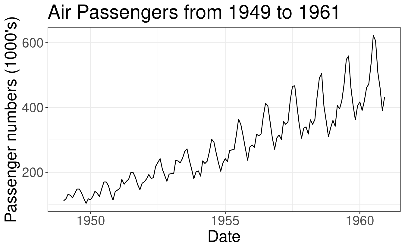
5.5.2.1 Rolling origin
The rolling origin cross-validation scheme lends itself to “online” learning algorithms, in which large streams of data have to be fit continually (respecting time), where the fit of the learning algorithm is (constantly) updated as more data accrues. In general, the rolling origin scheme defines an initial training set, and, with each iteration, the size of the training set grows by a batch of \(m\) observations, the size of the validation set remains constant, there might be a gap between training and validation times of size \(h\) (a lag window), and new folds are added until time \(t\) is reached in the validation set. The time points included in the training set always lag behind behind those in the validation set.
To further illustrate rolling origin cross-validation, we show below an example that yields three folds. Here, the first window size is fifteen time points, on which we first train the candidate learning algorithm. We then evaluate its performance on ten time points with a gap (\(h\)) of five time points between the training and validation sets.
In the following, we train the learning algorithm on a longer stream of data, 25 time points, including the original fifteen with which we initially started. Then, we evaluate its performance at a (temporal) distance ten time points ahead.
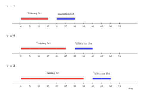
FIGURE 5.1: Rolling origin CV
We illustrate the usage of the rolling origin cross-validation scheme with
origami below, using the folds_rolling_origin(n, first_window, validation_size, gap, batch) function. In order to set up
folds_rolling_origin(n, first_window, validation_size, gap, batch), we need
the following,
- the total number of time points we wish to cross-validate (
n); - the size of the first training set (
first_window); - the size of the validation set (
validation_size); - the gap between training and validation set(
gap); and - the size of the training set update per iteration of cross-validation (
batch).
Our time-series has \(t=144\) time points. Setting first_window to \(50\),
validation_size to 10, gap to 5, and batch to 20 yields four time-series
folds; we show the first two below.
folds <- folds_rolling_origin(
  n = t,
  first_window = 50, validation_size = 10, gap = 5, batch = 20
)
folds[[1]]
$v
[1] 1

$training_set
 [1]  1  2  3  4  5  6  7  8  9 10 11 12 13 14 15 16 17 18 19 20 21 22 23 24 25
[26] 26 27 28 29 30 31 32 33 34 35 36 37 38 39 40 41 42 43 44 45 46 47 48 49 50

$validation_set
 [1] 56 57 58 59 60 61 62 63 64 65

attr(,"class")
[1] "fold"
folds[[2]]
$v
[1] 2

$training_set
 [1]  1  2  3  4  5  6  7  8  9 10 11 12 13 14 15 16 17 18 19 20 21 22 23 24 25
[26] 26 27 28 29 30 31 32 33 34 35 36 37 38 39 40 41 42 43 44 45 46 47 48 49 50
[51] 51 52 53 54 55 56 57 58 59 60 61 62 63 64 65 66 67 68 69 70

$validation_set
 [1] 76 77 78 79 80 81 82 83 84 85

attr(,"class")
[1] "fold"
5.5.2.2 Rolling window
Rather than adding more and more time points to the training set in each iteration of cross-validation (as under the rolling origin scheme), the rolling window cross-validation scheme “rolls” the training sample forward in time by \(m\) units (of time). This strategy can be useful, for example, in settings with parametric learning algorithms, which are often very sensitive to moment (e.g., mean, variance) or parameter drift, which is itself challenging to explicitly account for in the model construction step. The rolling window scheme is also computationally more efficient, and possibly warranted over rolling origin when working in streaming data analysis where the training data is too large for convenient access. In contrast to the rolling origin scheme, the sampled units in the training set are always the same for each iteration of the rolling window scheme.
The illustration below depicts rolling window cross-validation using three time-series folds. The first window size is 15 time points, on which we first train the candidate learning algorithm. As in the previous illustration, we evaluate its performance on 10 time points, with a gap of size 5 time points between the training and validation sets. However, for the next fold, we train the learning algorithm on time points further away from the origin (here, 10 time points). Note that the size of the training set in the new fold is the same as in the first fold (both include 15 time points). This setup keeps the training sets comparable over time (and across folds), unlike under the rolling origin cross-validation scheme. We then evaluate the performance of the candidate learning algorithm on 10 time points in the future.
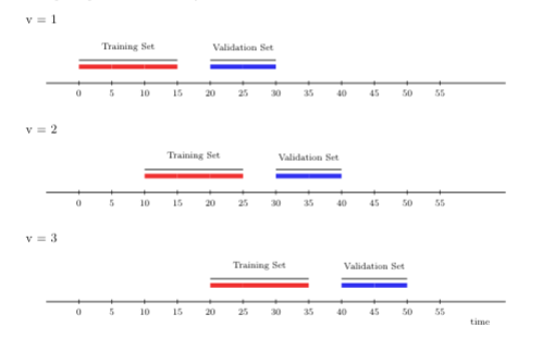
FIGURE 5.2: Rolling window CV
We demonstrate the usage of the rolling window cross-validation scheme with
origami below, using the folds_rolling_window(n, window_size, validation_size, gap, batch) function. In order to set up
folds_rolling_window(n, window_size, validation_size, gap, batch), we need to
specify the following arguments:
- the total number of time points we wish to cross-validate (
n); - the size of the training sets (
window_size); - the size of the validation set (
validation_size); - the gap between training and validation set (
gap); and - the size of the training set update per iteration of cross-validation (
batch).
Setting the window_size to \(50\), validation_size to 10, gap to 5 and
batch to 20, we also get 4 time-series folds; we show the first two below.
folds <- folds_rolling_window(
  n = t,
  window_size = 50, validation_size = 10, gap = 5, batch = 20
)
folds[[1]]
$v
[1] 1

$training_set
 [1]  1  2  3  4  5  6  7  8  9 10 11 12 13 14 15 16 17 18 19 20 21 22 23 24 25
[26] 26 27 28 29 30 31 32 33 34 35 36 37 38 39 40 41 42 43 44 45 46 47 48 49 50

$validation_set
 [1] 56 57 58 59 60 61 62 63 64 65

attr(,"class")
[1] "fold"
folds[[2]]
$v
[1] 2

$training_set
 [1] 21 22 23 24 25 26 27 28 29 30 31 32 33 34 35 36 37 38 39 40 41 42 43 44 45
[26] 46 47 48 49 50 51 52 53 54 55 56 57 58 59 60 61 62 63 64 65 66 67 68 69 70

$validation_set
 [1] 76 77 78 79 80 81 82 83 84 85

attr(,"class")
[1] "fold"
5.5.2.3 Rolling origin with \(V\)-fold
A variant of the rolling origin cross-validation scheme, accounting for sample
dependence, is the rolling-origin-\(V\)-fold cross-validation scheme. In contrast
to the canonical rolling origin scheme, under this hybrid scheme, sampled units
in the training and validation sets are not the same, which this scheme
accomplishes by incorporating \(V\)-fold cross-validation within the time-series
setup. Here, the learning algorithm’s predictions are evaluated on the future
time points of the time-series observational units excluded from the training
step, accommodating potential dependence not only across time but also across
observational units. To use the rolling-origin-\(V\)-fold cross-validation scheme
with origami, we can invoke the folds_vfold_rolling_origin_pooled(n, t, id, time, V, first_window, validation_size, gap, batch) function. In the figure
below, we show \(V=2\) folds, alongside two time-series (rolling origin)
cross-validation folds.
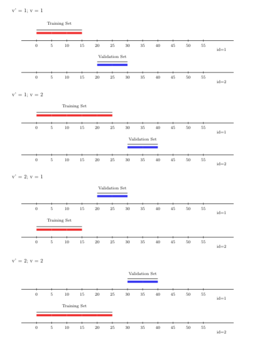
FIGURE 5.3: Rolling origin V-fold CV
5.5.2.4 Rolling window with \(V\)-fold
Just like the scheme described above, the rolling window approach, like the
rolling origin approach, can be extended to support multiple time-series with
arbitrary sample-level dependence by incorporating a \(V\)-fold splitting
component. This rolling-window-\(V\)-fold cross-validation scheme can be used
through origami via the folds_vfold_rolling_window_pooled(n, t, id, time, V, window_size, validation_size, gap, batch) function. The figure below displays
\(V=2\) folds and two time-series (rolling window) cross-validation folds.
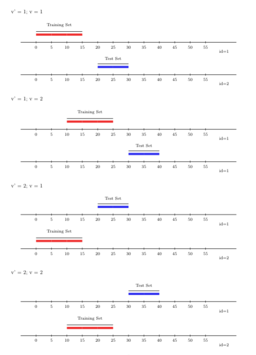
FIGURE 5.4: Rolling window V-fold CV
5.6 General workflow of origami
Before we dive into more details, let’s take a moment to review some of the
basic functionality in the origami R package. The main workhorse function in
origami is cross_validate(). To start off, the user must define the fold
structure and a function that operates on each fold (this cv_fun(), in
origami’s parlance, usually dictates how the candidate learning algorithm is
trained and its predictions validated).
Once passed to cross_validate(), the workhorse function will iteratively apply
the specified function (i.e., cv_fun()) to each fold, combining the
fold-specific results in a meaningful way. We will see this in action in later
sections — for now, we provide specific details on each each step of this
process below.
5.6.1 (1) Define folds
The folds object passed to cross_validate is a list of folds; such list
objects are generated using the make_folds() helper function. Each fold
consists of a list with a "training" index vector, a "validation" index
vector, and a "fold_index" (its order in the overall list of folds). The
make_folds() function supports a variety of cross-validation schemes,
described in the preceding section. The make_folds() function can also ensure
balance across levels of a given variable (through the strata_ids arguments),
and it can also keep all observations on the same independent unit together (via
the cluster_ids argument).
5.6.2 (2) Define the fold function
The cv_fun argument to cross_validate() is a custom function that performs
some operation on each fold (again, usually this specifies the training of the
candidate learning algorithm and its evaluation on a given training/validation
split, i.e., in a single fold). The first argument to this function is the
fold, which specifies the indices of the units in a given training/validation
split (note that this first argument is automatically passed to the cv_fun()
by cross_validate(), which queries the folds object from make_folds() in
doing so). Additional arguments can be passed to the cv_fun() through the
... argument to cross_validate(). Within this function, the convenience
functions training(), validation() and fold_index() can be used to return
the various components of a fold object. When the training() or
validation() functions are passed an object of a particular class, they will
index that object in a sensible way. For instance, if the input object is a
vector, these helper functions will index the vector directly, but if the input
object is a data.frame or matrix, these functions will automatically index
the rows. This allows the user to easily partition data into training and
validation sets. The fold function must return a named list of results
containing whatever fold-specific outputs are desired.
5.6.3 (3) Apply cross_validate()
After defining the folds, the cross_validate() function can be used to map the
cv_fun() across the folds; internally, this uses either lapply() or
future_lapply() (a parallelized variant of the same). In this way,
cross_validate() can be easily parallelized by specifying a parallelization
scheme (i.e., a plan from the future parallelization framework for
R (Bengtsson, 2021)). The
application of cross_validate() generates a list of results, matching the
customized list specified in the relevant cv_fun(). As noted above, each
call to cv_fun() itself returns a list of results, with different named
slots for each type of result we wish to store. The main cross_validate()
loop generates a list of these individual, fold-specific lists of results (a
list of lists or “meta-list”). Internally, this “meta-list” is cleaned up
(by concatenation) such that only a single slot per type of result specified by
the cv_fun() is returned (this too is a list of the results for each fold).
By default, the combine_results() helper function is used to combine the
individual, fold-specific lists of results in a sensible manner. How results
are combined is determined automatically by examining the data types of the
results from the first fold. This can be modified by specifying a list of
arguments in the .combine_control argument.
5.7 Cross-validation in action
We’ve waited long enough. Now, let’s see origami in action! In the next
chapter, we will learn how to use cross-validation with the Super Learner
algorithm, and how we can utilize the power of cross-validation to build optimal
ensembles of algorithms — going far beyond the application of cross-validation
to a single statistical learning method.
5.7.1 Cross-validation with linear regression
First, let’s load the relevant R packages, set a seed (for reproducibility),
and once again load the WASH Benefits example dataset. For illustrative
purposes, we’ll examine the application of cross-validation to simple linear
regression with origami, focusing on predicting the weight-for-height Z-score
(whz) using all of the other available covariates in the dataset. As mentioned
before, we will assume the dataset contains only independent and identically
distributed units, ignoring the clustering structure imposed by the trial
design. For the sake of illustration, we will work with only a subset of the
data, removing all observational units with missing covariate data from the
analysis-ready dataset. In the prior chapter, we discussed how to deal with
missingness.
library(stringr)
library(dplyr)
library(tidyr)

# load data set and take a peek
washb_data <- fread(
  paste0(
    "https://raw.githubusercontent.com/tlverse/tlverse-data/master/",
    "wash-benefits/washb_data.csv"
  ),
  stringsAsFactors = TRUE
)

# remove missing data with drop_na(), then pick just the first 500 rows
washb_data <- washb_data %>%
  drop_na() %>%
  slice(1:500)

# specify the outcome and covariates as character vectors
outcome <- "whz"
covars <- colnames(washb_data)[-which(names(washb_data) == outcome)]
Here’s a look at the data:
| whz | tr | fracode | month | aged | sex | momage | momedu | momheight | hfiacat | Nlt18 | Ncomp | watmin | elec | floor | walls | roof | asset_wardrobe | asset_table | asset_chair | asset_khat | asset_chouki | asset_tv | asset_refrig | asset_bike | asset_moto | asset_sewmach | asset_mobile |
|---|---|---|---|---|---|---|---|---|---|---|---|---|---|---|---|---|---|---|---|---|---|---|---|---|---|---|---|
| 0.00 | Control | N05265 | 9 | 268 | male | 30 | Primary (1-5y) | 146.4 | Food Secure | 3 | 11 | 0 | 1 | 0 | 1 | 1 | 0 | 1 | 1 | 1 | 0 | 1 | 0 | 0 | 0 | 0 | 1 |
| -1.16 | Control | N05265 | 9 | 286 | male | 25 | Primary (1-5y) | 148.8 | Moderately Food Insecure | 2 | 4 | 0 | 1 | 0 | 1 | 1 | 0 | 1 | 0 | 1 | 1 | 0 | 0 | 0 | 0 | 0 | 1 |
| -1.05 | Control | N08002 | 9 | 264 | male | 25 | Primary (1-5y) | 152.2 | Food Secure | 1 | 10 | 0 | 0 | 0 | 1 | 1 | 0 | 0 | 1 | 0 | 1 | 0 | 0 | 0 | 0 | 0 | 1 |
| -1.26 | Control | N08002 | 9 | 252 | female | 28 | Primary (1-5y) | 140.2 | Food Secure | 3 | 5 | 0 | 1 | 0 | 1 | 1 | 1 | 1 | 1 | 1 | 0 | 0 | 0 | 1 | 0 | 0 | 1 |
| -0.59 | Control | N06531 | 9 | 336 | female | 19 | Secondary (>5y) | 150.9 | Food Secure | 2 | 7 | 0 | 1 | 0 | 1 | 1 | 1 | 1 | 1 | 1 | 1 | 0 | 0 | 0 | 0 | 0 | 1 |
| -0.51 | Control | N06531 | 9 | 304 | male | 20 | Secondary (>5y) | 154.2 | Severely Food Insecure | 0 | 3 | 1 | 1 | 0 | 1 | 1 | 0 | 0 | 0 | 0 | 1 | 0 | 0 | 0 | 0 | 0 | 1 |
Let’s remind ourselves of the covariates to be used in the prediction step:
covars
 [1] "tr"             "fracode"        "month"          "aged"
 [5] "sex"            "momage"         "momedu"         "momheight"
 [9] "hfiacat"        "Nlt18"          "Ncomp"          "watmin"
[13] "elec"           "floor"          "walls"          "roof"
[17] "asset_wardrobe" "asset_table"    "asset_chair"    "asset_khat"
[21] "asset_chouki"   "asset_tv"       "asset_refrig"   "asset_bike"
[25] "asset_moto"     "asset_sewmach"  "asset_mobile"
Next, let’s fit a simple main-terms linear regression model to the
analysis-ready dataset. Here, our goal is to predict the weight-for-height
Z-score ("whz", which we assigned to the variable outcome) using all of the
available covariate data. Let’s try it out:
lm_mod <- lm(whz ~ ., data = washb_data)
summary(lm_mod)

Call:
lm(formula = whz ~ ., data = washb_data)

Residuals:
    Min      1Q  Median      3Q     Max
-2.8890 -0.6799 -0.0169  0.6595  3.1005

Coefficients:
                                Estimate Std. Error t value Pr(>|t|)
(Intercept)                     -1.89006    1.72022   -1.10   0.2725
trHandwashing                   -0.25276    0.17032   -1.48   0.1385
trNutrition                     -0.09695    0.15696   -0.62   0.5371
trNutrition + WSH               -0.09587    0.16528   -0.58   0.5622
trSanitation                    -0.27702    0.15846   -1.75   0.0811 .
trWSH                           -0.02846    0.15967   -0.18   0.8586
trWater                         -0.07148    0.15813   -0.45   0.6515
fracodeN05160                    0.62355    0.30719    2.03   0.0430 *
fracodeN05265                    0.38762    0.31011    1.25   0.2120
fracodeN05359                    0.10187    0.31329    0.33   0.7452
fracodeN06229                    0.30933    0.29766    1.04   0.2993
fracodeN06453                    0.08066    0.30006    0.27   0.7882
fracodeN06458                    0.43707    0.29970    1.46   0.1454
fracodeN06473                    0.45406    0.30912    1.47   0.1426
fracodeN06479                    0.60994    0.31463    1.94   0.0532 .
fracodeN06489                    0.25923    0.31901    0.81   0.4169
fracodeN06500                    0.07539    0.35794    0.21   0.8333
fracodeN06502                    0.36748    0.30504    1.20   0.2290
fracodeN06505                    0.20038    0.31560    0.63   0.5258
fracodeN06516                    0.55455    0.29807    1.86   0.0635 .
fracodeN06524                    0.49429    0.31423    1.57   0.1164
fracodeN06528                    0.75966    0.31060    2.45   0.0148 *
fracodeN06531                    0.36856    0.30155    1.22   0.2223
fracodeN06862                    0.56932    0.29293    1.94   0.0526 .
fracodeN08002                    0.36779    0.26846    1.37   0.1714
month                            0.17161    0.10865    1.58   0.1149
aged                            -0.00336    0.00112   -3.00   0.0029 **
sexmale                          0.12352    0.09203    1.34   0.1802
momage                          -0.01379    0.00973   -1.42   0.1570
momeduPrimary (1-5y)            -0.13214    0.15225   -0.87   0.3859
momeduSecondary (>5y)            0.12632    0.16041    0.79   0.4314
momheight                        0.00512    0.00919    0.56   0.5776
hfiacatMildly Food Insecure      0.05804    0.19341    0.30   0.7643
hfiacatModerately Food Insecure -0.01362    0.12887   -0.11   0.9159
hfiacatSeverely Food Insecure   -0.13447    0.25418   -0.53   0.5970
Nlt18                           -0.02557    0.04060   -0.63   0.5291
Ncomp                            0.00179    0.00762    0.23   0.8145
watmin                           0.01347    0.00861    1.57   0.1182
elec                             0.08906    0.10700    0.83   0.4057
floor                           -0.17763    0.17734   -1.00   0.3171
walls                           -0.03001    0.21445   -0.14   0.8888
roof                            -0.03716    0.49214   -0.08   0.9399
asset_wardrobe                  -0.05754    0.13736   -0.42   0.6755
asset_table                     -0.22079    0.12276   -1.80   0.0728 .
asset_chair                      0.28012    0.13750    2.04   0.0422 *
asset_khat                       0.02306    0.11766    0.20   0.8447
asset_chouki                    -0.13943    0.14084   -0.99   0.3227
asset_tv                         0.17723    0.12972    1.37   0.1726
asset_refrig                     0.12613    0.23162    0.54   0.5863
asset_bike                      -0.02568    0.10083   -0.25   0.7990
asset_moto                      -0.32094    0.19944   -1.61   0.1083
asset_sewmach                    0.05090    0.17795    0.29   0.7750
asset_mobile                     0.01420    0.14972    0.09   0.9245
---
Signif. codes:  0 '***' 0.001 '**' 0.01 '*' 0.05 '.' 0.1 ' ' 1

Residual standard error: 0.984 on 447 degrees of freedom
Multiple R-squared:  0.129, Adjusted R-squared:  0.0277
F-statistic: 1.27 on 52 and 447 DF,  p-value: 0.104
We can assess the quality of the model fit on the dataset by comparing the
linear model’s predictions of the weight-for-height Z-score against the
observations of the same in the dataset. This is the well-known, and standard,
mean squared error (MSE). We can extract this summary measure from the lm
model object like so
(err <- mean(resid(lm_mod)^2))
[1] 0.8657
The MSE estimate is 0.8657, which, from examination of the above, is merely the mean of the squared residuals of the model fit. An important problem arises when we assess the learning algorithm’s quality in this way — that is, because we have trained our linear regression model on the complete analysis-ready dataset and then assessed its performance (the MSE) on the same dataset, all of the data is used for both model training and validation. Unfortunately, this simple estimate of the MSE is overly optimistic. Why? The linear regression model is trained on the same dataset used in its evaluation, not unlike reusing problems from a homework assignment in a course examination. Of course, we are generally not interested in how well the algorithm explains variation in the observed dataset; rather, we are interested in how well the explanations provided by the learning algorithm generalize to a target population from which this particular sample is drawn. By using all of the data available to us for training the learning algorithm, we are left unable to honestly evaluate how well the algorithm fits (and, thus, explains) variation at the level of the target population. To resolve this issue, cross-validation allows for a particular procedure (e.g., linear regression) to be implemented over training and validation splits of the dataset, evaluating how well the procedure fits on a holdout (or validation) set. This evaluation of the learning algorithm’s quality on data unseen during the training phase provides an honest evaluation of the algorithm’s generalization error.
We can easily incorporate cross-validation into our linear regression procedure
using origami. First, let’s define a new function to perform linear regression
on a specific partition of the dataset (i.e., a fold):
cv_lm <- function(fold, data, reg_form) {
  # get name and index of outcome variable from regression formula
  out_var <- as.character(unlist(str_split(reg_form, " "))[1])
  out_var_ind <- as.numeric(which(colnames(data) == out_var))

  # split up data into training and validation sets
  train_data <- training(data)
  valid_data <- validation(data)

  # fit linear model on training set and predict on validation set
  mod <- lm(as.formula(reg_form), data = train_data)
  preds <- predict(mod, newdata = valid_data)
  valid_data <- as.data.frame(valid_data)

  # capture results to be returned as output
  out <- list(
    coef = data.frame(t(coef(mod))),
    SE = (preds - valid_data[, out_var_ind])^2
  )
  return(out)
}
Our cv_lm() function is quite simple: It merely splits the available data into
distinct training and validation sets (using the eponymous functions provided in
origami), fits the linear model on the training set, and evaluates the quality
of the trained linear regression model on the validation set. This is a simple
example of what origami considers to be a cv_fun() — functions for applying
a particular routine over an input dataset in cross-validated manner.
Having defined such a function, we can simply generate a set of partitions using
origami’s make_folds() function and apply our cv_lm() function over the
resultant folds object using cross_validate(). Below, we replicate the
re-substitution estimate of the error — we did this “by hand” above — using the
functions make_folds() and cv_lm().
# re-substitution estimate
resub <- make_folds(washb_data, fold_fun = folds_resubstitution)[[1]]
resub_results <- cv_lm(fold = resub, data = washb_data, reg_form = "whz ~ .")
mean(resub_results$SE, na.rm = TRUE)
[1] 0.8657
This (nearly) matches the estimate of the error that we obtained above.
We can more honestly evaluate the error by \(V\)-fold cross-validation, which
partitions the dataset into \(V\) subsets, fitting the algorithm on \(V - 1\) of the
subsets (training) and evaluating on the subset that was held out from
fitting (validation). This is repeated such that each holdout subset
takes a turn being used for validation. We can easily apply our cv_lm()
function in this way using origami’s cross_validate() (note that by default
this function performs \(10\)-fold cross-validation):
# cross-validated estimate
folds <- make_folds(washb_data)
cvlm_results <- cross_validate(
  cv_fun = cv_lm, folds = folds, data = washb_data, reg_form = "whz ~ .",
  use_future = FALSE
)
mean(cvlm_results$SE, na.rm = TRUE)
[1] 1.35
Having performed \(V\)-fold cross-validation with 10 folds (the default), we quickly notice that our previous estimate of the model error (by re-substitution) was a bit optimistic. The honest estimate of the linear regression model’s error is larger!
5.7.2 Cross-validation with random forests
To examine origami further, let’s return to our example analysis using the
WASH Benefits dataset. Here, we will write a new cv_fun() function. As an
example, we will use Breiman’s random forest algorithm (Breiman, 2001),
implemented in the randomForest() function (from the randomForest package):
# make sure to load the package!
library(randomForest)

cv_rf <- function(fold, data, reg_form) {
  # get name and index of outcome variable from regression formula
  out_var <- as.character(unlist(str_split(reg_form, " "))[1])
  out_var_ind <- as.numeric(which(colnames(data) == out_var))

  # define training and validation sets based on input object of class "folds"
  train_data <- training(data)
  valid_data <- validation(data)

  # fit Random Forest regression on training set and predict on holdout set
  mod <- randomForest(formula = as.formula(reg_form), data = train_data)
  preds <- predict(mod, newdata = valid_data)
  valid_data <- as.data.frame(valid_data)

  # define output object to be returned as list (for flexibility)
  out <- list(
    coef = data.frame(mod$coefs),
    SE = ((preds - valid_data[, out_var_ind])^2)
  )
  return(out)
}
The cv_rf() function, which cross-validates the training and evaluation of the
randomForest algorithm, used our previous cv_lm() function as a template.
For now, individual cv_fun()s must be written by hand; however, in future
releases of the package, a wrapper may be made available to support
auto-generating cv_funs for use with origami.
Below, we use cross_validate() to apply our custom cv_rf() function over the
folds object generated by make_folds():
# now, let's cross-validate...
folds <- make_folds(washb_data)
cvrf_results <- cross_validate(
  cv_fun = cv_rf, folds = folds,
  data = washb_data, reg_form = "whz ~ .",
  use_future = FALSE
)
mean(cvrf_results$SE)
[1] 1.027
Using \(V\)-fold cross-validation with 10 folds, we obtain an honest estimate of
the prediction error of this random forest. This is one example of how
origami’s cross_validate() procedure can be generalized to arbitrary
estimation techniques, as long as an appropriate cv_fun() function is
available.
5.7.3 Cross-validation with ARIMA
Cross-validation can also be used for the selection of forecasting models in
settings with time-series data. Here, the partitioning scheme mirrors the
application of the forecasting model: We’ll train the learning algorithm on past
observations (either all available or a recent, in time, subset), and then use
the fitted model to predict the next (again, in time) few observations. To
demonstrate this, we return to the AirPassengers dataset, a monthly
time-series of passenger air traffic for thousands of travelers.
data(AirPassengers)
print(AirPassengers)
     Jan Feb Mar Apr May Jun Jul Aug Sep Oct Nov Dec
1949 112 118 132 129 121 135 148 148 136 119 104 118
1950 115 126 141 135 125 149 170 170 158 133 114 140
1951 145 150 178 163 172 178 199 199 184 162 146 166
1952 171 180 193 181 183 218 230 242 209 191 172 194
1953 196 196 236 235 229 243 264 272 237 211 180 201
1954 204 188 235 227 234 264 302 293 259 229 203 229
1955 242 233 267 269 270 315 364 347 312 274 237 278
1956 284 277 317 313 318 374 413 405 355 306 271 306
1957 315 301 356 348 355 422 465 467 404 347 305 336
1958 340 318 362 348 363 435 491 505 404 359 310 337
1959 360 342 406 396 420 472 548 559 463 407 362 405
1960 417 391 419 461 472 535 622 606 508 461 390 432
Suppose we want to pick between two forecasting models with different ARIMA (AutoRegressive Integrated Moving Average) model configurations. We can choose among such models by evaluating their forecasting performance. First, we set up an appropriate cross-validation scheme for use with time-series data. Here, we pick the rolling origin cross-validation scheme described above.
folds <- make_folds(AirPassengers,
  fold_fun = folds_rolling_origin,
  first_window = 36, validation_size = 24, batch = 10
)

# How many folds where generated?
length(folds)
[1] 9

# Examine the first 2 folds.
folds[[1]]
$v
[1] 1

$training_set
 [1]  1  2  3  4  5  6  7  8  9 10 11 12 13 14 15 16 17 18 19 20 21 22 23 24 25
[26] 26 27 28 29 30 31 32 33 34 35 36

$validation_set
 [1] 37 38 39 40 41 42 43 44 45 46 47 48 49 50 51 52 53 54 55 56 57 58 59 60

attr(,"class")
[1] "fold"
folds[[2]]
$v
[1] 2

$training_set
 [1]  1  2  3  4  5  6  7  8  9 10 11 12 13 14 15 16 17 18 19 20 21 22 23 24 25
[26] 26 27 28 29 30 31 32 33 34 35 36 37 38 39 40 41 42 43 44 45 46

$validation_set
 [1] 47 48 49 50 51 52 53 54 55 56 57 58 59 60 61 62 63 64 65 66 67 68 69 70

attr(,"class")
[1] "fold"
By default, folds_rolling_origin will increase the size of the training set by
one time point in each training fold. Had we followed the default option, we
would have 85 folds to train! Luckily, we can pass the batch as an option to
folds_rolling_origin, telling it to increase the size of the training set by
10 points in each iteration (so that we don’t have so many training folds).
Since we want to forecast the immediately following time point, the gap
argument remains at its default of zero.
# make sure to load the package!
library(forecast)

# function to calculate cross-validated squared error
cv_forecasts <- function(fold, data) {
  # Get training and validation data
  train_data <- training(data)
  valid_data <- validation(data)
  valid_size <- length(valid_data)

  train_ts <- ts(log10(train_data), frequency = 12)

  # First arima model
  arima_fit <- arima(train_ts, c(0, 1, 1),
    seasonal = list(
      order = c(0, 1, 1),
      period = 12
    )
  )
  raw_arima_pred <- predict(arima_fit, n.ahead = valid_size)
  arima_pred <- 10^raw_arima_pred$pred
  arima_MSE <- mean((arima_pred - valid_data)^2)

  # Second arima model
  arima_fit2 <- arima(train_ts, c(5, 1, 1),
    seasonal = list(
      order = c(0, 1, 1),
      period = 12
    )
  )
  raw_arima_pred2 <- predict(arima_fit2, n.ahead = valid_size)
  arima_pred2 <- 10^raw_arima_pred2$pred
  arima_MSE2 <- mean((arima_pred2 - valid_data)^2)

  out <- list(mse = data.frame(
    fold = fold_index(),
    arima = arima_MSE, arima2 = arima_MSE2
  ))
  return(out)
}

mses <- cross_validate(
  cv_fun = cv_forecasts, folds = folds, data = AirPassengers,
  use_future = FALSE
)
mses$mse
  fold   arima arima2
1    1   68.21  137.3
2    2  319.68  313.2
3    3  578.35  713.4
4    4  428.69  505.3
5    5  407.33  371.3
6    6  281.82  251.0
7    7  827.56  910.1
8    8 2099.59 2213.1
9    9  398.37  293.4
colMeans(mses$mse[, c("arima", "arima2")])
 arima arima2
 601.1  634.2
By applying cross_validate() with this cv_forecasts() custom function, we
find that the ARIMA model with no AR (autoregressive) component seems to be a
better fit for this dataset.
5.8 Exercises
5.8.1 Review of Key Concepts
Compare and contrast \(V\)-fold cross-validation with re-substitution cross-validation. What are some of the differences between the two methods? How are they similar? Describe a scenario when you would use one over the other.
-
What are the advantages and disadvantages of \(V\)-fold cross-validation relative to:
- holdout cross-validation?
- leave-one-out cross-validation?
Why is \(V\)-fold cross-validation inappropriate for use with time-series data?
Would you use rolling window or rolling origin cross-validation for non-stationary time-series? Why? ### The Ideas in Action
Let \(Y\) be a binary variable with \(P(Y=1 \mid W) = 0.01\), that is, a rare outcome. What kind of cross-validation scheme should be used with this type of outcome? How can we do this with the
origamipackage?Consider the WASH Benefits example dataset discussed in this chapter. How can we incorporate cluster-level information into a cross-validation scheme? How can we implement this strategy with the
origamipackage?
5.8.2 Advanced Topics
Think about a dataset with a spatial dependence structure, in which the degree of dependence is known such that the groups formed by this dependence structure are clear and where there are no spillover effects. What kind of cross-validation scheme would be appropriate in this case?
Continuing from the previous problem, what kind of procedure, and cross-validation scheme, can we use if the spatial dependence is not as clearly defined as in assumptions made in the preceding problem?
-
Consider a classification problem with a large number of predictors and a binary outcome. Your friendly neighborhood statistician proposes the following analysis:
- First, screen the predictors, isolating only those covariates that are strongly correlated with the (binary) outcome labels.
- Next, train a learning algorithm using only this subset of covariates that are highly correlated with the outcome.
- Finally, use cross-validation to estimate the tuning parameters and the performance of the learning algorithm.
Is this application of cross-validation correct? Why or why not?