6 Super Learning
Rachael Phillips
Based on the sl3 R package by Jeremy
Coyle, Nima Hejazi, Ivana Malenica, Rachael Phillips, and Oleg Sofrygin.
Learning Objectives
By the end of this chapter you will be able to:
Select a performance metric that is optimized by the true prediction function, or define the true prediction prediction of interest as the optimizer of the performance metric.
-
Assemble a diverse set (“library”) of learners to be considered in the super learner. In particular, you should be able to:
- Customize a learner by modifying its tuning parameters.
- Create variations of the same base learner with different tuning parameter specifications.
- Couple screener(s) with learner(s) to create learners that consider as covariates a reduced, screener-selected subset of them.
Specify a meta-learner that optimizes the objective function of interest.
Justify the library and the meta-learner in terms of the prediction problem at hand, intended use of the analysis in the real world, statistical model, sample size, number of covariates, and outcome prevalence for discrete outcomes.
Interpret the fit for a super learner from the table of cross-validated risk estimates and the super learner coefficients.
6.1 Introduction
A common task in data analysis is prediction, or using the observed data to learn a function that takes as input data on covariates/predictors and outputs a predicted value. Occasionally, the scientific question of interest lends itself to causal effect estimation. Even in these scenarios, where prediction is not in the forefront, prediction tasks are embedded in the procedure. For instance, in targeted minimum loss-based estimation (TMLE) for the average treatment effect, predictive modeling is necessary for estimating outcome regressions and propensity scores.
There are various strategies that can be employed to model relationships from data, which we refer to interchangeably as “estimators”, “algorithms”, and “learners”. For some data, algorithms that can pick up on complex relationships among variables are necessary to adequately model it. For other data, parametric regression learners might fit the data reasonably well. It is generally impossible to know in advance which approach will be the best for a given data set and prediction problem.
The Super Learner (SL) solves the issue of selecting an algorithm, as it can
consider many of them - from the simplest parametric regressions to the most
complex machine learning algorithms (e.g., neural nets, support vector machines,
etc). Additionally, it is proven to perform as well as possible
(as good as the unknown oracle) in large samples, given the learners specified
(Dudoit and van der Laan, 2005; van der Laan et al., 2004; van der Laan and Dudoit, 2003; van der Vaart et al., 2006).
The SL represents an entirely pre-specified, flexible, and theoretically
grounded approach for predictive modeling. It has been shown to be adaptive and
robust in a variety of applications, even in very small samples. Detailed
descriptions outlining the SL procedure are widely available (Naimi and Balzer, 2018; Polley and van der Laan, 2010). Practical considerations for specifying the SL, including
how to specify a rich and diverse library of learners, choose a performance
metric for the SL, and specify a cross-validation (CV) scheme, are described in
a pre-print article (Phillips et al., 2023). Here, we focus on introducing sl3, the
standard tlverse software package for SL.
6.2 How to Fit the Super Learner
In this section, the core functionality for fitting any SL with sl3 is
illustrated. In the sections that follow, additional sl3 functionality is
presented.
Fitting any SL with sl3 consists of the following three steps:
- Define the prediction task with
make_sl3_Task. - Instantiate the SL with
Lrnr_sl. - Fit the SL to the task with
train.
Running example with WASH Benefits dataset
We will use the WASH Benefits Bangladesh study as an example to guide this
overview of sl3. In this study, we are interested in predicting the child
development outcome, weight-for-height z-score, from covariates/predictors,
including socio-economic status variables, gestational age, and maternal
features. More information on this dataset is described in the “Meet the
Data” chapter of the
tlverse handbook.
Preliminaries
First, we need to load the data and relevant packages into the R session.
Load the data
We will use the fread function in the data.table R package to load the WASH
Benefits example dataset:
washb_data <- fread(
  paste0(
    "https://raw.githubusercontent.com/tlverse/tlverse-data/master/",
    "wash-benefits/washb_data.csv"
  ),
  stringsAsFactors = TRUE
)
Next, we will take a peek at the first few rows of our dataset:
head(washb_data)| whz | tr | fracode | month | aged | sex | momage | momedu | momheight | hfiacat | Nlt18 | Ncomp | watmin | elec | floor | walls | roof | asset_wardrobe | asset_table | asset_chair | asset_khat | asset_chouki | asset_tv | asset_refrig | asset_bike | asset_moto | asset_sewmach | asset_mobile |
|---|---|---|---|---|---|---|---|---|---|---|---|---|---|---|---|---|---|---|---|---|---|---|---|---|---|---|---|
| 0.00 | Control | N05265 | 9 | 268 | male | 30 | Primary (1-5y) | 146.4 | Food Secure | 3 | 11 | 0 | 1 | 0 | 1 | 1 | 0 | 1 | 1 | 1 | 0 | 1 | 0 | 0 | 0 | 0 | 1 |
| -1.16 | Control | N05265 | 9 | 286 | male | 25 | Primary (1-5y) | 148.8 | Moderately Food Insecure | 2 | 4 | 0 | 1 | 0 | 1 | 1 | 0 | 1 | 0 | 1 | 1 | 0 | 0 | 0 | 0 | 0 | 1 |
| -1.05 | Control | N08002 | 9 | 264 | male | 25 | Primary (1-5y) | 152.2 | Food Secure | 1 | 10 | 0 | 0 | 0 | 1 | 1 | 0 | 0 | 1 | 0 | 1 | 0 | 0 | 0 | 0 | 0 | 1 |
| -1.26 | Control | N08002 | 9 | 252 | female | 28 | Primary (1-5y) | 140.2 | Food Secure | 3 | 5 | 0 | 1 | 0 | 1 | 1 | 1 | 1 | 1 | 1 | 0 | 0 | 0 | 1 | 0 | 0 | 1 |
| -0.59 | Control | N06531 | 9 | 336 | female | 19 | Secondary (>5y) | 150.9 | Food Secure | 2 | 7 | 0 | 1 | 0 | 1 | 1 | 1 | 1 | 1 | 1 | 1 | 0 | 0 | 0 | 0 | 0 | 1 |
| -0.51 | Control | N06531 | 9 | 304 | male | 20 | Secondary (>5y) | 154.2 | Severely Food Insecure | 0 | 3 | 1 | 1 | 0 | 1 | 1 | 0 | 0 | 0 | 0 | 1 | 0 | 0 | 0 | 0 | 0 | 1 |
Install sl3 software (as needed)
To install any package, we recommend first clearing the R workspace and then restarting the R session. In RStudio, this can be achieved by clicking the tab “Session” then “Clear Workspace”, and then clicking “Session” again then “Restart R”.
We can install sl3 using the function install_github provided in the
devtools R package. We are using the development (“devel”) version of sl3
in these materials, so we show how to install that version below.
library(devtools)
install_github("tlverse/sl3@devel")
Once the R package is installed, we recommend restarting the R session again.
1. Define the prediction task with make_sl3_Task
The sl3_Task object defines the prediction task of interest. Recall that
our task in this illustrative example is to use the WASH Benefits Bangladesh
example dataset to learn a function of the covariates for predicting
weight-for-height Z-score whz.
# create the task (i.e., use washb_data to predict outcome using covariates)
task <- make_sl3_Task(
  data = washb_data,
  outcome = "whz",
  covariates = c("tr", "fracode", "month", "aged", "sex", "momage", "momedu",
                 "momheight", "hfiacat", "Nlt18", "Ncomp", "watmin", "elec",
                 "floor", "walls", "roof", "asset_wardrobe", "asset_table",
                 "asset_chair", "asset_khat", "asset_chouki", "asset_tv",
                 "asset_refrig", "asset_bike", "asset_moto", "asset_sewmach",
                 "asset_mobile")
)

# let's examine the task
task
An sl3 Task with 4695 obs and these nodes:
$covariates
 [1] "tr"              "fracode"         "month"           "aged"
 [5] "sex"             "momage"          "momedu"          "momheight"
 [9] "hfiacat"         "Nlt18"           "Ncomp"           "watmin"
[13] "elec"            "floor"           "walls"           "roof"
[17] "asset_wardrobe"  "asset_table"     "asset_chair"     "asset_khat"
[21] "asset_chouki"    "asset_tv"        "asset_refrig"    "asset_bike"
[25] "asset_moto"      "asset_sewmach"   "asset_mobile"    "delta_momage"
[29] "delta_momheight"

$outcome
[1] "whz"

$id
NULL

$weights
NULL

$offset
NULL

$time
NULL
The sl3_Task keeps track of the roles the variables play in the prediction
problem. Additional information relevant to the prediction task (such as
observational-level weights, offset, id, CV folds) can also be specified in
make_sl3_Task. The default CV fold structure in sl3 is V-fold CV (VFCV)
with V=10 folds. If id is specified in the task, a clustered V=10 VFCV
scheme is considered; if the outcome type is binary or categorical, then
a stratified V=10 VFCV scheme is considered. Different CV schemes can be
specified by inputting an origami folds object, as generated by the
make_folds function in the origami R package. For more information,
refer to the previous Chapter on cross-validation, or consult documentation
on origami’s make_folds function (e.g., in RStudio, by
loading the origami R package and then inputting “?make_folds” in the
Console). For more details on sl3_Task, refer to its documentation (e.g., by
inputting “?sl3_Task” in R).
Tip: If you type task$ and then press the tab key (press tab twice if not in
RStudio), you can view all of the active and public fields, as well as methods that
can be accessed from the task$ object. This $ is like the key to access
many internals of an object. In the next section, will see how we can use $
to dig into SL fit objects as well - to obtain predictions from an SL fit or
candidate learners, examine an SL fit or its candidates, and summarize an SL
fit.
2. Instantiate the Super Learner with Lrnr_sl
In order to create Lrnr_sl we need to specify, at the minimum, a set of
learners for the SL to consider as candidates. This set of algorithms is
also commonly referred to as the “library”. We might also specify the
meta-learner, which is the algorithm that ensembles the learners (note that this part is
optional since there are already defaults set up in sl3). See “Practical
considerations for specifying a super learner” for step-by-step guidelines for
tailoring the SL specification (including the library and meta-learner(s)) that optimizes the prediction task at hand (Phillips et al., 2023).
Learners have properties that indicate what features they support. We may use
the sl3_list_properties() function to get a list of all properties supported
by at least one learner:
sl3_list_properties()
 [1] "binomial"      "categorical"   "continuous"    "cv"
 [5] "density"       "h2o"           "ids"           "importance"
 [9] "offset"        "preprocessing" "sampling"      "screener"
[13] "timeseries"    "weights"       "wrapper"
Since whz is a continuous outcome, we can identify the learners that support
this outcome type with sl3_list_learners():
sl3_list_learners(properties = "continuous")
 [1] "Lrnr_arima"                     "Lrnr_bartMachine"
 [3] "Lrnr_bayesglm"                  "Lrnr_bilstm"
 [5] "Lrnr_bound"                     "Lrnr_caret"
 [7] "Lrnr_cv_selector"               "Lrnr_dbarts"
 [9] "Lrnr_earth"                     "Lrnr_expSmooth"
[11] "Lrnr_ga"                        "Lrnr_gam"
[13] "Lrnr_gbm"                       "Lrnr_glm"
[15] "Lrnr_glm_fast"                  "Lrnr_glm_semiparametric"
[17] "Lrnr_glmnet"                    "Lrnr_glmtree"
[19] "Lrnr_grf"                       "Lrnr_gru_keras"
[21] "Lrnr_gts"                       "Lrnr_h2o_glm"
[23] "Lrnr_h2o_grid"                  "Lrnr_hal9001"
[25] "Lrnr_HarmonicReg"               "Lrnr_hts"
[27] "Lrnr_lightgbm"                  "Lrnr_lstm_keras"
[29] "Lrnr_mean"                      "Lrnr_multiple_ts"
[31] "Lrnr_nnet"                      "Lrnr_nnls"
[33] "Lrnr_optim"                     "Lrnr_pkg_SuperLearner"
[35] "Lrnr_pkg_SuperLearner_method"   "Lrnr_pkg_SuperLearner_screener"
[37] "Lrnr_polspline"                 "Lrnr_randomForest"
[39] "Lrnr_ranger"                    "Lrnr_rpart"
[41] "Lrnr_rugarch"                   "Lrnr_screener_correlation"
[43] "Lrnr_solnp"                     "Lrnr_stratified"
[45] "Lrnr_svm"                       "Lrnr_tsDyn"
[47] "Lrnr_xgboost"
Now that we have an idea of some learners, let’s instantiate a few of them.
Below we instantiate Lrnr_glm and Lrnr_mean, a main terms generalized
linear model (GLM) and a mean model, respectively.
For both of the learners created above, we just used the default tuning parameters. We can also customize a learner’s tuning parameters to incorporate a diversity of different settings, and consider the same learner with different tuning parameter specifications.
Below, we consider the same base learner, Lrnr_glmnet (i.e., GLMs
with elastic net regression), and create two different candidates from it:
an L2-penalized/ridge regression and an L1-penalized/lasso regression.
# penalized regressions:
lrn_ridge <- Lrnr_glmnet$new(alpha = 0)
lrn_lasso <- Lrnr_glmnet$new(alpha = 1)
By setting alpha in Lrnr_glmnet above, we customized this learner’s tuning
parameter. When we instantiate Lrnr_hal9001 below we show how multiple tuning
parameters (specifically, max_degreeand num_knots) can be modified at the
same time.
Let’s also instantiate some more learners that do not enforce relationships to be linear or monotonic, which further diversifies the set of candidates to include nonparametric learners.
# spline regressions:
lrn_polspline <- Lrnr_polspline$new()
lrn_earth <- Lrnr_earth$new()

# fast highly adaptive lasso (HAL) implementation
lrn_hal <- Lrnr_hal9001$new(max_degree = 2, num_knots = c(3,2), nfolds = 5)

# tree-based methods
lrn_ranger <- Lrnr_ranger$new()
lrn_xgb <- Lrnr_xgboost$new()
Let’s also include a generalized additive model (GAM) and Bayesian GLM to further diversify the pool that we will consider as candidates in the SL.
lrn_gam <- Lrnr_gam$new()
lrn_bayesglm <- Lrnr_bayesglm$new()
Now that we’ve instantiated a set of learners, we need to put them together so
the SL can consider them as candidates. In sl3, we do this by creating a
so-called Stack of learners. A Stack is created in the same way we
created the learners. This is because Stack is a learner itself; it has the
same interface as all of the other learners. What makes a stack special is that
it considers multiple learners at once: it can train them simultaneously, so
that their predictions can be combined and/or compared.
stack <- Stack$new(
  lrn_glm, lrn_mean, lrn_ridge, lrn_lasso, lrn_polspline, lrn_earth, lrn_hal,
  lrn_ranger, lrn_xgb, lrn_gam, lrn_bayesglm
)
stack
 [1] "Lrnr_glm_TRUE"
 [2] "Lrnr_mean"
 [3] "Lrnr_glmnet_NULL_deviance_10_0_100_TRUE"
 [4] "Lrnr_glmnet_NULL_deviance_10_1_100_TRUE"
 [5] "Lrnr_polspline"
 [6] "Lrnr_earth_2_3_backward_0_1_0_0"
 [7] "Lrnr_hal9001_2_1_c(3, 2)_5"
 [8] "Lrnr_ranger_500_TRUE_none_1"
 [9] "Lrnr_xgboost_20_1"
[10] "Lrnr_gam_NULL_NULL_GCV.Cp"
[11] "Lrnr_bayesglm_TRUE"
We can see that the names of the learners in the stack are long. This is
because the default naming of a learner in sl3 is clunky: for each learner,
every tuning parameter in sl3 is contained in the name. In the next section,
“Naming
Learners”,
we show a few different ways for the user to name learners as they wish.
Now that we have instantiated a set of learners and stacked them together, we
are ready to instantiate the SL. We will use the default meta-learner, which is
non-negative least squares (NNLS) regression (Lrnr_nnls) for continuous
outcomes. For illustrative purposes, we will still go ahead and specify it
in the following.
3. Fit the Super Learner to the prediction task with train
The last step for fitting the SL to the prediction task is to call train and
supply the task. Before we call train, we will set a random number generator
so the results are reproducible, and we will also time it.
start_time <- proc.time() # start time

set.seed(4197)
sl_fit <- sl$train(task = task)

runtime_sl_fit <- proc.time() - start_time # end time - start time = run time
runtime_sl_fit
   user  system elapsed
280.831   6.176 277.401
It took 277.4 seconds (4.6 minutes) to fit the SL.
Summary
In this section, the core functionality for fitting any SL with sl3 was
illustrated. This consists of the following three steps:
- Define the prediction task with
make_sl3_Task. - Instantiate the SL with
Lrnr_sl. - Fit the SL to the task with
train.
This example was for demonstrative purposes only. See Phillips et al. (2023) for step-by-step guidelines for constructing a SL that is well-specified for the prediction task at hand.
6.3 Obtaining Predictions
6.3.1 Super learner and candidate learner predictions
We will draw on the fitted SL object from above, sl_fit, to obtain the
SL’s predicted whz value for each subject.
sl_preds <- sl_fit$predict(task = task)
head(sl_preds)
[1] -0.5719 -0.8717 -0.6881 -0.7342 -0.6308 -0.6596
We can also obtain predicted values from a candidate learner in the SL. Below we obtain predictions for the GLM learner.
glm_preds <- sl_fit$learner_fits$Lrnr_glm_TRUE$predict(task = task)
head(glm_preds)
[1] -0.7262 -0.9361 -0.7085 -0.6492 -0.7013 -0.8462
Note that the predicted values for the SL correspond to so-called “full fits”
of the candidate learners, in which the candidates are fit to the entire
analytic dataset, i.e., all of the data supplied as data to make_sl3_Task.
Figure 2 in Phillips et al. (2023) provides a visual overview of the SL fitting
procedure.
# we can also access the candidate learner full fits directly and obtain
# the same "full fit" candidate predictions from there
# (we split this into two lines to avoid overflow)
stack_full_fits <- sl_fit$fit_object$full_fit$learner_fits$Stack$learner_fits
glm_preds_full_fit <- stack_full_fits$Lrnr_glm_TRUE$predict(task)

# check that they are identical
identical(glm_preds, glm_preds_full_fit)
[1] TRUE
Below we visualize the observed values for whz and predicted whz values for
SL, GLM and the mean.
# table of observed and predicted outcome values and arrange by observed values
df_plot <- data.table(
  Obs = washb_data[["whz"]], SL_Pred = sl_preds, GLM_Pred = glm_preds,
  Mean_Pred = sl_fit$learner_fits$Lrnr_mean$predict(task)
)
df_plot <- df_plot[order(df_plot$Obs), ]
head(df_plot)| Obs | SL_Pred | GLM_Pred | Mean_Pred |
|---|---|---|---|
| -4.67 | -1.487 | -0.9096 | -0.5861 |
| -4.18 | -1.170 | -0.6391 | -0.5861 |
| -4.17 | -1.147 | -0.8098 | -0.5861 |
| -4.03 | -1.447 | -0.8960 | -0.5861 |
| -3.95 | -1.579 | -1.1952 | -0.5861 |
| -3.90 | -1.285 | -0.9849 | -0.5861 |
# melt the table so we can plot observed and predicted values
df_plot$id <- seq(1:nrow(df_plot))
df_plot_melted <- melt(
  df_plot, id.vars = "id",
  measure.vars = c("Obs", "SL_Pred", "GLM_Pred", "Mean_Pred")
)

library(ggplot2)
ggplot(df_plot_melted, aes(id, value, color = variable)) +
  geom_point(size = 0.1) +
  labs(x = "Subjects (ordered by increasing whz)",
       y = "whz") +
  theme(legend.position = "bottom", legend.title = element_blank(),
        axis.text.x = element_blank(), axis.ticks.x = element_blank()) +
  guides(color = guide_legend(override.aes = list(size = 1)))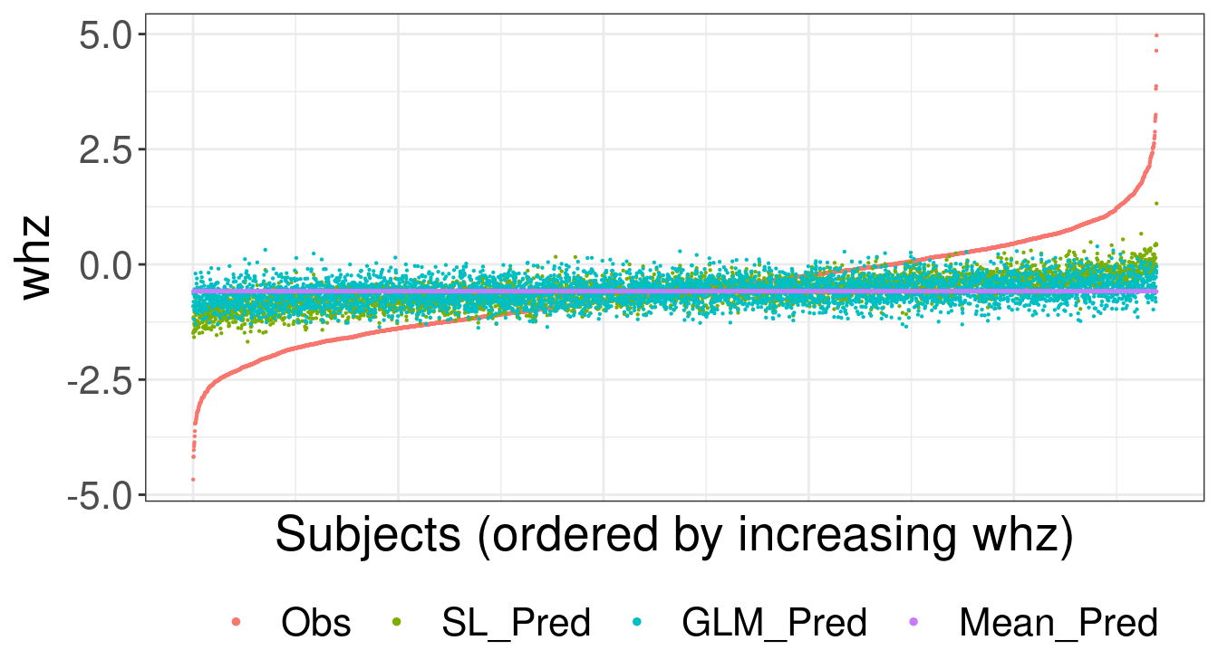
FIGURE 6.1: Observed and predicted values for weight-for-height z-score (whz)
6.3.2 Cross-validated predictions
We can also obtain the cross-validated (CV) predictions for the candidate learners. We can do this in a few different ways.
# one way to obtain the CV predictions for the candidate learners
cv_preds_option1 <- sl_fit$fit_object$cv_fit$predict_fold(
  task = task, fold_number = "validation"
)
# another way to obtain the CV predictions for the candidate learners
cv_preds_option2 <- sl_fit$fit_object$cv_fit$predict(task = task)

# we can check that they are identical
identical(cv_preds_option1, cv_preds_option2)
[1] TRUE
head(cv_preds_option1)| Lrnr_glm_TRUE | Lrnr_mean | Lrnr_glmnet_NULL_deviance_10_0_100_TRUE | Lrnr_glmnet_NULL_deviance_10_1_100_TRUE | Lrnr_polspline | Lrnr_earth_2_3_backward_0_1_0_0 | Lrnr_hal9001_2_1_c(3, 2)_5 | Lrnr_ranger_500_TRUE_none_1 | Lrnr_xgboost_20_1 | Lrnr_gam_NULL_NULL_GCV.Cp | Lrnr_bayesglm_TRUE |
|---|---|---|---|---|---|---|---|---|---|---|
| -0.7453 | -0.5931 | -0.6949 | -0.7034 | -0.7250 | -0.7156 | -0.6967 | -0.7419 | -0.7883 | -0.7244 | -0.7452 |
| -0.9447 | -0.5865 | -0.8150 | -0.7789 | -0.8449 | -0.8352 | -0.8333 | -0.6542 | -0.5983 | -0.9324 | -0.9445 |
| -0.6494 | -0.5931 | -0.7004 | -0.7254 | -0.7140 | -0.6089 | -0.6887 | -0.6391 | -0.6453 | -0.6111 | -0.6495 |
| -0.6211 | -0.5846 | -0.6237 | -0.6594 | -0.6525 | -0.6916 | -0.6843 | -0.6278 | -0.4697 | -0.5910 | -0.6214 |
| -0.7647 | -0.5846 | -0.6711 | -0.7069 | -0.7001 | -0.6969 | -0.6788 | -0.5657 | -0.6588 | -0.7975 | -0.7649 |
| -0.8873 | -0.5763 | -0.8106 | -0.7578 | -0.7125 | -0.4770 | -0.7393 | -0.8545 | -0.6963 | -0.9132 | -0.8872 |
predict_fold
Our first option to get CV predictions, cv_preds_option1, used the
predict_fold function to obtain validation set predictions across all folds.
This function only exists for learner fits that are cross-validated in sl3,
like those in Lrnr_sl. In addition to supplying fold_number = "validation"
in predict_fold, we can set fold_number = "full" to obtain predictions from
learners fit to the entire analytic dataset (i.e., all of the data supplied to
make_sl3_Task). For instance, below we show that glm_preds we calculated
above can also be obtained by setting fold_number = "full".
full_fit_preds <- sl_fit$fit_object$cv_fit$predict_fold(
  task = task, fold_number = "full"
)
glm_full_fit_preds <- full_fit_preds$Lrnr_glm_TRUE

# check that they are identical
identical(glm_preds, glm_full_fit_preds)
[1] TRUE
We can also supply a specific integer between 1 and the number of CV folds
to the fold_number argument in predict_fold; example of this
functionality is shown in the next part.
Cross-validated predictions by hand
We can get the CV predictions “by hand”, by tapping into each of the folds, and then using the fitted candidate learners (which were trained to the training set for each fold) to predict validation set outcomes (which were not seen in training).
##### CV predictions "by hand" #####
# for each fold, i, we obtain validation set predictions:
cv_preds_list <- lapply(seq_along(task$folds), function(i){

  # get validation dataset for fold i:
  v_data <- task$data[task$folds[[i]]$validation_set, ]

  # get observed outcomes in fold i's validation dataset:
  v_outcomes <- v_data[["whz"]]

  # make task (for prediction) using fold i's validation dataset as data,
  # and keeping all else the same:
  v_task <- make_sl3_Task(covariates = task$nodes$covariates, data = v_data)

  # get predicted outcomes for fold i's validation dataset, using candidates
  # trained to fold i's training dataset
  v_preds <- sl_fit$fit_object$cv_fit$predict_fold(
    task = v_task, fold_number = i
  )
  # note: v_preds is a matrix of candidate learner predictions, where the
  # number of rows is the number of observations in fold i's validation dataset
  # and the number of columns is the number of candidate learners (excluding
  # any that might have failed)

  # an identical way to get v_preds, which is used when we calculate the
  # cv risk by hand in a later part of this chapter:
  # v_preds <- sl_fit$fit_object$cv_fit$fit_object$fold_fits[[i]]$predict(
  #   task = v_task
  # )

  # we will also return the row indices for fold i's validation set, so we
  # can later reorder the CV predictions and make sure they are equal to what
  # we obtained above
  return(list("v_preds" = v_preds, "v_index" = task$folds[[i]]$validation_set))
})

# extract the validation set predictions across all folds
cv_preds_byhand <- do.call(rbind, lapply(cv_preds_list, "[[", "v_preds"))

# extract the indices of validation set observations across all folds
# then reorder cv_preds_byhand to correspond to the ordering in the data
row_index_in_data <- unlist(lapply(cv_preds_list, "[[", "v_index"))
cv_preds_byhand_ordered <- cv_preds_byhand[order(row_index_in_data), ]
# now we can check that they are identical
identical(cv_preds_option1, cv_preds_byhand_ordered)
[1] TRUE
6.3.3 Predictions with new data
If we wanted to obtain predicted values for new data then we would need to
create a new sl3_Task from the new data. Also, the covariates in this new
sl3_Task must be identical to the covariates in the sl3_Task for training.
As an example, let’s assume we have new covariate data washb_data_new for
which we want to use the fitted SL to obtain predicted weight-for-height
z-score values.
# we do not evaluate this code chunk, as `washb_data_new` does not exist
prediction_task <- make_sl3_Task(
  data = washb_data_new, # assuming we have some new data for predictions
  covariates = c("tr", "fracode", "month", "aged", "sex", "momage", "momedu",
                 "momheight", "hfiacat", "Nlt18", "Ncomp", "watmin", "elec",
                 "floor", "walls", "roof", "asset_wardrobe", "asset_table",
                 "asset_chair", "asset_khat", "asset_chouki", "asset_tv",
                 "asset_refrig", "asset_bike", "asset_moto", "asset_sewmach",
                 "asset_mobile")
)
sl_preds_new_task <- sl_fit$predict(task = prediction_task)
6.3.4 Counterfactual predictions
Counterfactual predictions are predicted values under an intervention of
interest. Recall from above that we can obtain predicted values for new data by
creating a sl3_Task with the new data whose covariates match the set
considered for training. As an example that draws on the WASH Benefits
Bangladesh study, suppose we would like to obtain predictions for every
subject’s weight-for-height z-score (whz) outcome under an intervention on
treatment (tr) that sets it to the nutrition, water, sanitation, and
handwashing regime.
First we need to create a copy of the dataset, and then we can intervene on
tr in the copied dataset, create a new sl3_Task using the copied data and
the same covariates as the training task, and finally obtain predictions
from the fitted SL (which we named sl_fit in the previous section).
### 1. Copy data
tr_intervention_data <- data.table::copy(washb_data)

### 2. Define intervention in copied dataset
tr_intervention <- rep("Nutrition + WSH", nrow(washb_data))
# NOTE: When we intervene on a categorical variable (such as "tr"), we need to
#       define the intervention as a categorical variable (ie a factor).
#       Also, even though not all levels of the factor will be represented in
#       the intervention, we still need this factor to reflect all of the
#       levels that are present in the observed data
tr_levels <- levels(washb_data[["tr"]])
tr_levels
[1] "Control"         "Handwashing"     "Nutrition"       "Nutrition + WSH"
[5] "Sanitation"      "WSH"             "Water"
tr_intervention <- factor(tr_intervention, levels = tr_levels)
tr_intervention_data[,"tr" := tr_intervention, ]

### 3. Create a new sl3_Task
# note that we do not need to specify the outcome in this new task since we are
# only using it to obtain predictions
tr_intervention_task <- make_sl3_Task(
  data = tr_intervention_data,
  covariates = c("tr", "fracode", "month", "aged", "sex", "momage", "momedu",
                 "momheight", "hfiacat", "Nlt18", "Ncomp", "watmin", "elec",
                 "floor", "walls", "roof", "asset_wardrobe", "asset_table",
                 "asset_chair", "asset_khat", "asset_chouki", "asset_tv",
                 "asset_refrig", "asset_bike", "asset_moto", "asset_sewmach",
                 "asset_mobile")
)
### 4. Get predicted values under intervention of interest
# SL predictions of what "whz" would have been had everyone received "tr"
# equal to "Nutrition + WSH"
counterfactual_pred <- sl_fit$predict(tr_intervention_task)
Note that this type of intervention, where every subject receives the same intervention, is referred to as “static”. Interventions that vary depending on the characteristics of the subject are referred to as “dynamic”. For instance, we might consider an intervention that sets the treatment to the desired (nutrition, water, sanitation, and handwashing) regime if the subject has a refridgerator, and a nutrition-omitted (water, sanitation, and handwashing) regime otherwise.
dynamic_tr_intervention_data <- data.table::copy(washb_data)

dynamic_tr_intervention <- ifelse(
  washb_data[["asset_refrig"]] == 1, "Nutrition + WSH", "WSH"
)
dynamic_tr_intervention <- factor(dynamic_tr_intervention, levels = tr_levels)
dynamic_tr_intervention_data[,"tr" := dynamic_tr_intervention, ]

dynamic_tr_intervention_task <- make_sl3_Task(
  data = dynamic_tr_intervention_data,
  covariates = c("tr", "fracode", "month", "aged", "sex", "momage", "momedu",
                 "momheight", "hfiacat", "Nlt18", "Ncomp", "watmin", "elec",
                 "floor", "walls", "roof", "asset_wardrobe", "asset_table",
                 "asset_chair", "asset_khat", "asset_chouki", "asset_tv",
                 "asset_refrig", "asset_bike", "asset_moto", "asset_sewmach",
                 "asset_mobile")
)
### 4. Get predicted values under intervention of interest
# SL predictions of what "whz" would have been had every subject received "tr"
# equal to "Nutrition + WSH" if they had a fridge and "WSH" if they didn't have
# a fridge
counterfactual_pred <- sl_fit$predict(dynamic_tr_intervention_task)
6.4 Summarizing Super Learner Fits
6.4.1 Super Learner coefficients / fitted meta-learner summary
We can see how the meta-learner created a function of the learners in a few ways. In our illustrative example, we considered the default, NNLS meta-learner for continuous outcomes. For meta-learners that simply learn a weighted combination, we can examine their coefficients.
round(sl_fit$coefficients, 3)
                          Lrnr_glm_TRUE                               Lrnr_mean
                                  0.000                                   0.000
Lrnr_glmnet_NULL_deviance_10_0_100_TRUE Lrnr_glmnet_NULL_deviance_10_1_100_TRUE
                                  0.096                                   0.000
                         Lrnr_polspline         Lrnr_earth_2_3_backward_0_1_0_0
                                  0.168                                   0.399
             Lrnr_hal9001_2_1_c(3, 2)_5             Lrnr_ranger_500_TRUE_none_1
                                  0.000                                   0.337
                      Lrnr_xgboost_20_1               Lrnr_gam_NULL_NULL_GCV.Cp
                                  0.000                                   0.000
                     Lrnr_bayesglm_TRUE
                                  0.000
We can also examine the coefficients by directly accessing the meta-learner’s fit object.
metalrnr_fit <- sl_fit$fit_object$cv_meta_fit$fit_object
round(metalrnr_fit$coefficients, 3)
                          Lrnr_glm_TRUE                               Lrnr_mean
                                  0.000                                   0.000
Lrnr_glmnet_NULL_deviance_10_0_100_TRUE Lrnr_glmnet_NULL_deviance_10_1_100_TRUE
                                  0.096                                   0.000
                         Lrnr_polspline         Lrnr_earth_2_3_backward_0_1_0_0
                                  0.168                                   0.399
             Lrnr_hal9001_2_1_c(3, 2)_5             Lrnr_ranger_500_TRUE_none_1
                                  0.000                                   0.337
                      Lrnr_xgboost_20_1               Lrnr_gam_NULL_NULL_GCV.Cp
                                  0.000                                   0.000
                     Lrnr_bayesglm_TRUE
                                  0.000
Direct access to the meta-learner fit object is also handy for more complex meta-learners (e.g., non-parametric meta-learners) that are not defined by a simple set of main terms regression coefficients.
6.4.2 Cross-validated predictive performance
We can obtain a table of the cross-validated (CV) predictive performance, i.e., the CV risk, for each learner included in the SL. Below, we use the squared error loss for the evaluation function, which equates to the mean squared error (MSE) as the metric to summarize predictive performance. The reason why we use the MSE is because it is a valid metric for estimating the conditional mean, which is what we’re learning the prediction function for in the WASH Benefits example. For more information on selecting an appropriate performance metric, see Phillips et al. (2023).
cv_risk_table <- sl_fit$cv_risk(eval_fun = loss_squared_error)
cv_risk_table[,c(1:3)]| learner | coefficients | MSE |
|---|---|---|
| Lrnr_glm_TRUE | 0.0000 | 1.022 |
| Lrnr_mean | 0.0000 | 1.065 |
| Lrnr_glmnet_NULL_deviance_10_0_100_TRUE | 0.0957 | 1.017 |
| Lrnr_glmnet_NULL_deviance_10_1_100_TRUE | 0.0000 | 1.015 |
| Lrnr_polspline | 0.1678 | 1.016 |
| Lrnr_earth_2_3_backward_0_1_0_0 | 0.3993 | 1.013 |
| Lrnr_hal9001_2_1_c(3, 2)_5 | 0.0000 | 1.018 |
| Lrnr_ranger_500_TRUE_none_1 | 0.3372 | 1.014 |
| Lrnr_xgboost_20_1 | 0.0000 | 1.079 |
| Lrnr_gam_NULL_NULL_GCV.Cp | 0.0000 | 1.024 |
| Lrnr_bayesglm_TRUE | 0.0000 | 1.022 |
Cross-validated predictive performance by hand
Similar to how we got the CV predictions “by hand”, we can also calculate the CV
performance/risk in a way that exposes the procedure. Specifically, this is done
by tapping into each of the folds, and then using the fitted candidate learners
(which were trained to the training set for each fold) to predict validation set
outcomes (which were not seen in training) and then measure the predictive
performance (i.e., risk). Each candidate learner’s fold-specific risk is then
averaged across all folds to obtain the CV risk. The function cv_risk does
all of this internally and we show how to do it by hand below, which can be
helpful for understanding the CV risk and how it is calculated.
##### CV risk "by hand" #####
# for each fold, i, we obtain predictive performance/risk for each candidate:
cv_risks_list <- lapply(seq_along(task$folds), function(i){

  # get validation dataset for fold i:
  v_data <- task$data[task$folds[[i]]$validation_set, ]

  # get observed outcomes in fold i's validation dataset:
  v_outcomes <- v_data[["whz"]]

  # make task (for prediction) using fold i's validation dataset as data,
  # and keeping all else the same:
  v_task <- make_sl3_Task(covariates = task$nodes$covariates, data = v_data)

  # get predicted outcomes for fold i's validation dataset, using candidates
  # trained to fold i's training dataset
  v_preds <- sl_fit$fit_object$cv_fit$fit_object$fold_fits[[i]]$predict(v_task)
  # note: v_preds is a matrix of candidate learner predictions, where the
  # number of rows is the number of observations in fold i's validation dataset
  # and the number of columns is the number of candidate learners (excluding
  # any that might have failed)

  # calculate predictive performance for fold i for each candidate
  eval_function <- loss_squared_error # valid for estimation of conditional mean
  v_losses <- apply(v_preds, 2, eval_function, v_outcomes)
  cv_risks <- colMeans(v_losses)
  return(cv_risks)
})
# average the predictive performance across all folds for each candidate
cv_risks_byhand <- colMeans(do.call(rbind, cv_risks_list))
cv_risk_table_byhand <- data.table(
  learner = names(cv_risks_byhand), MSE = cv_risks_byhand
)
# check that the CV risks are identical when calculated by hand and function
# (ignoring small differences by rounding to the fourth decimal place)
identical(
  round(cv_risk_table_byhand$MSE,4), round(as.numeric(cv_risk_table$MSE),4)
)
[1] TRUE
6.4.3 Cross-validated Super Learner
We can see from the CV risk table above that the SL is not listed. This is
because we do not have a CV risk for the SL unless we cross-validate it or
include it as a candidate in another SL; the latter is shown in the next
subsection.
Below, we show how to obtain a CV risk estimate for the SL using function
cv_sl. Like before when we called sl$train, we will set a random number
generator so the results are reproducible, and we will also time this.
start_time <- proc.time()

set.seed(569)
cv_sl_fit <- cv_sl(lrnr_sl = sl_fit, task = task, eval_fun = loss_squared_error)

runtime_cv_sl_fit <- proc.time() - start_time
runtime_cv_sl_fit
user system elapsed
2792.6 159.6 3051.4 It took 3051.4 seconds (50.9 minutes) to fit the CV SL.
cv_sl_fit$cv_risk[,c(1:3)]| learner | MSE | se |
|---|---|---|
| Lrnr_glm_TRUE | 1.022 | 0.0240 |
| Lrnr_mean | 1.065 | 0.0250 |
| Lrnr_glmnet_NULL_deviance_10_0_100_TRUE | 1.017 | 0.0237 |
| Lrnr_glmnet_NULL_deviance_10_1_100_TRUE | 1.014 | 0.0236 |
| Lrnr_polspline | 1.016 | 0.0237 |
| Lrnr_earth_2_3_backward_0_1_0_0 | 1.013 | 0.0235 |
| Lrnr_hal9001_2_1_c(3, 2)_5 | 1.018 | 0.0237 |
| Lrnr_ranger_500_TRUE_none_1 | 1.014 | 0.0236 |
| Lrnr_xgboost_20_1 | 1.079 | 0.0248 |
| Lrnr_gam_NULL_NULL_GCV.Cp | 1.024 | 0.0239 |
| Lrnr_bayesglm_TRUE | 1.022 | 0.0240 |
| SuperLearner | 1.007 | 0.0234 |
The CV risk of the SL is 0.0234, which is lower than all of the candidates’ CV risks.
We can see how the SL fits varied across the folds by the coefficients for the SL on each fold.
round(cv_sl_fit$coef, 3)| fold | Lrnr_glm_TRUE | Lrnr_mean | Lrnr_glmnet_NULL_deviance_10_0_100_TRUE | Lrnr_glmnet_NULL_deviance_10_1_100_TRUE | Lrnr_polspline | Lrnr_earth_2_3_backward_0_1_0_0 | Lrnr_hal9001_2_1_c(3, 2)_5 | Lrnr_ranger_500_TRUE_none_1 | Lrnr_xgboost_20_1 | Lrnr_gam_NULL_NULL_GCV.Cp | Lrnr_bayesglm_TRUE |
|---|---|---|---|---|---|---|---|---|---|---|---|
| 1 | 0.000 | 0 | 0.047 | 0.000 | 0.243 | 0.253 | 0.000 | 0.456 | 0.000 | 0.000 | 0 |
| 2 | 0.000 | 0 | 0.000 | 0.257 | 0.161 | 0.000 | 0.071 | 0.473 | 0.038 | 0.000 | 0 |
| 3 | 0.000 | 0 | 0.030 | 0.000 | 0.079 | 0.175 | 0.147 | 0.415 | 0.000 | 0.154 | 0 |
| 4 | 0.050 | 0 | 0.000 | 0.459 | 0.000 | 0.111 | 0.020 | 0.360 | 0.000 | 0.000 | 0 |
| 5 | 0.000 | 0 | 0.075 | 0.275 | 0.000 | 0.315 | 0.000 | 0.318 | 0.000 | 0.017 | 0 |
| 6 | 0.025 | 0 | 0.248 | 0.000 | 0.110 | 0.351 | 0.000 | 0.267 | 0.000 | 0.000 | 0 |
| 7 | 0.000 | 0 | 0.000 | 0.236 | 0.114 | 0.084 | 0.139 | 0.406 | 0.000 | 0.020 | 0 |
| 8 | 0.189 | 0 | 0.007 | 0.000 | 0.196 | 0.029 | 0.207 | 0.372 | 0.000 | 0.000 | 0 |
| 9 | 0.113 | 0 | 0.000 | 0.103 | 0.106 | 0.129 | 0.000 | 0.548 | 0.000 | 0.000 | 0 |
| 10 | 0.000 | 0 | 0.000 | 0.185 | 0.000 | 0.154 | 0.000 | 0.661 | 0.000 | 0.000 | 0 |
6.4.4 Revere-cross-validated predictive performance of Super Learner
We can also use so-called “revere”, to obtain a partial CV risk for the SL,
where the SL candidate learner fits are cross-validated but the meta-learner fit
is not. It takes essentially no extra time to calculate a revere-CV
performance/risk estimate of the SL, since we already have the CV fits of the
candidates. This isn’t to say that revere-CV SL performance can replace that
obtained from actual CV SL. Revere can be used to very quickly examine an
approximate lower bound on the SL’s CV risk when the meta-learner is a simple
model, like NNLS. We can output the revere-based CV risk estimate by setting
get_sl_revere_risk = TRUE in cv_risk.
cv_risk_w_sl_revere <- sl_fit$cv_risk(
  eval_fun = loss_squared_error, get_sl_revere_risk = TRUE
)
cv_risk_w_sl_revere[,c(1:3)]| learner | coefficients | MSE |
|---|---|---|
| Lrnr_glm_TRUE | 0.0000 | 1.022 |
| Lrnr_mean | 0.0000 | 1.065 |
| Lrnr_glmnet_NULL_deviance_10_0_100_TRUE | 0.0957 | 1.017 |
| Lrnr_glmnet_NULL_deviance_10_1_100_TRUE | 0.0000 | 1.015 |
| Lrnr_polspline | 0.1678 | 1.016 |
| Lrnr_earth_2_3_backward_0_1_0_0 | 0.3993 | 1.013 |
| Lrnr_hal9001_2_1_c(3, 2)_5 | 0.0000 | 1.018 |
| Lrnr_ranger_500_TRUE_none_1 | 0.3372 | 1.014 |
| Lrnr_xgboost_20_1 | 0.0000 | 1.079 |
| Lrnr_gam_NULL_NULL_GCV.Cp | 0.0000 | 1.024 |
| Lrnr_bayesglm_TRUE | 0.0000 | 1.022 |
| SuperLearner | NA | 1.003 |
Revere-cross-validated predictive performance of Super Learner by hand
We show how to calculate the revere-CV predictive performance/risk of the SL by hand below, as this might be helpful for understanding revere and how it can be used to obtain a partial CV performance/risk estimate for the SL.
##### revere-based risk "by hand" #####
# for each fold, i, we obtain predictive performance/risk for the SL
sl_revere_risk_list <- lapply(seq_along(task$folds), function(i){
  # get validation dataset for fold i:
  v_data <- task$data[task$folds[[i]]$validation_set, ]

  # get observed outcomes in fold i's validation dataset:
  v_outcomes <- v_data[["whz"]]

  # make task (for prediction) using fold i's validation dataset as data,
  # and keeping all else the same:
  v_task <- make_sl3_Task(
    covariates = task$nodes$covariates, data = v_data
  )

  # get predicted outcomes for fold i's validation dataset, using candidates
  # trained to fold i's training dataset
  v_preds <- sl_fit$fit_object$cv_fit$fit_object$fold_fits[[i]]$predict(v_task)

  # make a metalevel task (for prediction with sl):
  v_meta_task <- make_sl3_Task(
    covariates = sl_fit$fit_object$cv_meta_task$nodes$covariates,
    data = v_preds
  )

  # get predicted outcomes for fold i's metalevel dataset, using the fitted
  # metalearner, cv_meta_fit
  sl_revere_v_preds <- sl_fit$fit_object$cv_meta_fit$predict(task=v_meta_task)
  # note: cv_meta_fit was trained on the metalevel dataset, which contains the
  # candidates' cv predictions and validation dataset outcomes across ALL folds,
  # so cv_meta_fit has already seen fold i's validation dataset outcomes.

  # calculate predictive performance for fold i for the SL
  eval_function <- loss_squared_error # valid for estimation of conditional mean
  # note: by evaluating the predictive performance of the SL using outcomes
  # that were already seen by the metalearner, this is not a cross-validated
  # measure of predictive performance for the SL.
  sl_revere_v_loss <- eval_function(
    pred = sl_revere_v_preds, observed = v_outcomes
  )
  sl_revere_v_risk <- mean(sl_revere_v_loss)
  return(sl_revere_v_risk)
})
# average the predictive performance across all folds for the SL
sl_revere_risk_byhand <- mean(unlist(sl_revere_risk_list))
sl_revere_risk_byhand
[1] 1.003

# check that our calculation by hand equals what is output in cv_risk_table_revere
sl_revere_risk <- as.numeric(cv_risk_w_sl_revere[learner=="SuperLearner","MSE"])
sl_revere_risk
[1] 1.003
The reason why this is not a fully cross-validated risk estimate is because the
cv_meta_fit object above (which is the trained meta-learner), was previously
fit to the entire matrix of CV predictions from every fold (i.e., the
meta-level dataset; see Figure 2 in Phillips et al. (2023) for more detail). This is why
revere-based risks are not a true CV risk. If the meta-learner is not a simple
regression function, and instead a more flexible learner (e.g., random
forest) is used as the meta-learner, then the revere-CV risk estimate of the
resulting SL will be a worse approximation of the CV risk estimate. This is
because more flexible learners are more likely to overfit. When simple
parametric regressions are used as a meta-learner, like what we considered in
our SL (NNLS with Lrnr_nnls), and like all of the default meta-learners in
sl3, then the revere-CV risk is a quick way to examine an approximation of
the CV risk estimate of the SL and it can thought of as a ballpark lower bound
on it. This idea holds in our example; that is, with the simple NNLS
meta-learner the revere risk estimate of the SL (1.0033)
is very close to, and slightly lower than, the CV risk estimate for the SL
(1.0067).
6.5 Discrete Super Learner
From the glossary (Table 1) entry for discrete SL (dSL) in Phillips et al. (2023),
the dSL is “a SL that uses a winner-take-all meta-learner called
the cross-validated selector. The dSL is therefore identical to the candidate
with the best cross-validated performance; its predictions will be the same as
this candidate’s predictions”. The cross-validated selector is
Lrnr_cv_selector in sl3 (see Lrnr_cv_selector documentation for more
detail) and a dSL is instantiated in sl3 by using Lrnr_cv_selector as the
meta-learner in Lrnr_sl.
cv_selector <- Lrnr_cv_selector$new(eval_function = loss_squared_error)
dSL <- Lrnr_sl$new(learners = stack, metalearner = cv_selector)
Just like before, we use the learner’s train method to fit it to the
prediction task.
set.seed(4197)
dSL_fit <- dSL$train(task)
Following from subsection “Summarizing Super Learner
Fits”
above, we can see how the Lrnr_cv_selector meta-learner created a function of
the candidates.
round(dSL_fit$coefficients, 3)
                          Lrnr_glm_TRUE                               Lrnr_mean
                                      0                                       0
Lrnr_glmnet_NULL_deviance_10_0_100_TRUE Lrnr_glmnet_NULL_deviance_10_1_100_TRUE
                                      0                                       0
                         Lrnr_polspline         Lrnr_earth_2_3_backward_0_1_0_0
                                      0                                       1
             Lrnr_hal9001_2_1_c(3, 2)_5             Lrnr_ranger_500_TRUE_none_1
                                      0                                       0
                      Lrnr_xgboost_20_1               Lrnr_gam_NULL_NULL_GCV.Cp
                                      0                                       0
                     Lrnr_bayesglm_TRUE
                                      0
We can also examine the CV risk of the candidates alongside the coefficients:
dSL_cv_risk_table <- dSL_fit$cv_risk(eval_fun = loss_squared_error)
dSL_cv_risk_table[,c(1:3)]| learner | coefficients | MSE |
|---|---|---|
| Lrnr_glm_TRUE | 0 | 1.022 |
| Lrnr_mean | 0 | 1.065 |
| Lrnr_glmnet_NULL_deviance_10_0_100_TRUE | 0 | 1.017 |
| Lrnr_glmnet_NULL_deviance_10_1_100_TRUE | 0 | 1.014 |
| Lrnr_polspline | 0 | 1.016 |
| Lrnr_earth_2_3_backward_0_1_0_0 | 1 | 1.013 |
| Lrnr_hal9001_2_1_c(3, 2)_5 | 0 | 1.018 |
| Lrnr_ranger_500_TRUE_none_1 | 0 | 1.013 |
| Lrnr_xgboost_20_1 | 0 | 1.079 |
| Lrnr_gam_NULL_NULL_GCV.Cp | 0 | 1.024 |
| Lrnr_bayesglm_TRUE | 0 | 1.022 |
The multivariate adaptive splines regression candidate (Lrnr_earth) has the
lowest CV risk. Indeed, our winner-take-all meta-learner Lrnr_cv_selector
gave it a weight of one and all others zero weight; the resulting dSL will be
defined by this weighted combination, i.e., dSL_fit will be identical to the
full fit Lrnr_earth. We verify that the dSL_fit’s predictions are identical
to Lrnr_earth’s below.
dSL_pred <- dSL_fit$predict(task)
earth_pred <- dSL_fit$learner_fits$Lrnr_earth_2_3_backward_0_1_0_0$predict(task)
identical(dSL_pred, earth_pred)
[1] TRUE
6.5.1 Including ensemble Super Learner(s) as candidate(s) in discrete Super Learner
We recommend using CV to evaluate the predictive performance of the SL. We
showed how to do this with cv_sl above. We have also seen that when we
include a learner as a candidate in the SL (in sl3 terms, when we include a
learner in the Stack passed to Lrnr_sl as learners), we are able to
examine its CV risk. Also, when we use the dSL, the candidate that achieved the
lowest CV risk defines the resulting SL. We therefore can use the dSL automate
a procedure for obtaining a final SL that represents the candidate with the
best cross-validated predictive performance. When the ensemble SL (eSL) and
its candidate learners are considered in a dSL as candidates, the eSL’s CV
performance can be compared to that from the learners from which it was
constructed, and the final SL will be the candidate that achieved the lowest CV
risk. From the glossary (Table 1) entry for eSL in Phillips et al. (2023), an
eSL is “a SL that uses any parametric or non-parametric algorithm as its
meta-learner. Therefore, the eSL is defined by a combination of multiple
candidates; its predictions are defined by a combination of multiple candidates’
predictions.” In the following, we show how to include the eSL, and multiple
eSLs, as candidates in the dSL.
Recall the SL object, sl, defined in section 2:
# in the section 2 we defined Lrnr_sl as
# sl <- Lrnr_sl$new(learners = stack, metalearner = Lrnr_nnls$new())
sl is an eSL since it used NNLS as the meta-learner. We rename sl to
eSL_metaNNLS below to clarify that this is an eSL that uses NNLS as its
meta-learner. Note that the candidate learners in this eSL are those passed
to the learners argument, i.e., stack.
# let's rename it to clarify that this is an eSL that uses NNLS as meta-learner
eSL_metaNNLS <- sl
To consider the eSL_metaNNLS as an additional candidate in stack, we can
create a new stack that includes the original candidate learners and the eSL.
stack_with_eSL <- Stack$new(stack, eSL_metaNNLS)To instantiate the dSL that considers as its candidates eSL_metaNNLS and the
individual learners from which eSL_metaNNLS was constructed, we define
a new Lrnr_sl that considers stack_with_eSL as candidates and
Lrnr_cv_selector as the meta-learner.
cv_selector <- Lrnr_cv_selector$new(eval_function = loss_squared_error)
dSL <- Lrnr_sl$new(learners = stack_with_eSL, metalearner = cv_selector)
When we include an eSL as a candidate in the dSL, this allows the eSL’s CV
performance to be compared to that from the other learners from which it was
constructed. This is similar to calling CV SL, cv_sl, above. The difference
between including the eSL as a candidate in the dSL and calling cv_sl is that
the former automates a procedure for the final SL to be the learner that
achieved the best CV predictive performance, i.e., lowest CV risk. If the eSL
outperforms any other candidate, the dSL will end up selecting it and the
resulting SL will be the eSL. As mentioned in Phillips et al. (2023), “another advantage
of this approach is that multiple eSLs that use more flexible meta-learner
methods (e.g., non-parametric machine learning algorithms like HAL) can be
evaluated simultaneously.”
Below, we show how multiple eSLs can be included as candidates in a dSL:
# instantiate more eSLs
eSL_metaNNLSconvex <- Lrnr_sl$new(
  learners = stack, metalearner = Lrnr_nnls$new(convex = TRUE)
)
eSL_metaLasso <- Lrnr_sl$new(learners = stack, metalearner = lrn_lasso)
eSL_metaEarth <- Lrnr_sl$new(learners = stack, metalearner = lrn_earth)
eSL_metaRanger <- Lrnr_sl$new(learners = stack, metalearner = lrn_ranger)
eSL_metaHAL <- Lrnr_sl$new(learners = stack, metalearner = lrn_hal)
# adding the eSLs to the stack that defined them
stack_with_eSLs <- Stack$new(
  stack, eSL_metaNNLS, eSL_metaNNLSconvex, eSL_metaLasso, eSL_metaEarth,
  eSL_metaRanger, eSL_metaHAL
)
# specify dSL
dSL <- Lrnr_sl$new(learners = stack_with_eSLs, metalearner = cv_selector)
We included as candidates in the dSL:
- the same eSL as before,
eSL_metaNNLS; - the learners considered as candidates in (1);
- an eSL that considered the same candidate learners as (1) and a convex combination-constrained NNLS as the meta-learner;
- an eSL that considered the same candidate learners as (1) and a lasso
meta-learner, using
lrn_lassowhich was instantiated in section 2; - an eSL that considered the same candidate learners as (1) and a
multivariate adaptive regression splines (earth) meta-learner, using
lrn_earthwhich was instantiated in section 2; - an eSL that considered the same candidate learners as (1) and a
ranger meta-learner, using
lrn_rangerwhich was instantiated in section 2; and - an eSL that considered the same candidate learners as (1) and a
HAL meta-learner, using
lrn_halwhich was instantiated in section 2.
Running this many eSLs in the dSL is currently very computationally intensive
in sl3, as it is akin to running cross-validated SL for each eSL. Parallel
programming (reviewed below) is recommended for training learners that are
computationally intensive, like the dSL defined above. That is, a parallel
processing scheme should be defined before calling dSL$train(task) in order
to speed up the run time.
6.6 Parallel Processing
It’s straightforward to take advantage of sl3’s built-in parallel processing
support, which draws on the future R
package, which
provides a lightweight, unified Future API for sequential and parallel
processing of R expressions via futures. From the future package
documentation: “This package implements sequential, multicore, multisession, and cluster futures. With these, R expressions can be evaluated on the local
machine, in parallel a set of local machines, or distributed on a mix of local
and remote machines. Extensions to this package implement additional backends
for processing futures via compute cluster schedulers, etc. Because of its
unified API, there is no need to modify any code in order switch from
sequential on the local machine to, say, distributed processing on a remote
compute cluster. Another strength of this package is that global variables and
functions are automatically identified and exported as needed, making it
straightforward to tweak existing code to make use of futures.”
To use future with sl3, you can simply choose a futures plan(), as shown
below.
# let's load the future package and set n-1 cores for parallel processing
library(future)
ncores <- availableCores()-1
ncores
system
     1
plan(multicore, workers = ncores)
# now, let's re-train sl in parallel for demonstrative purposes
# we will also set a stopwatch so we can see how long this takes
start_time <- proc.time()

set.seed(4197)
sl_fit_parallel <- sl$train(task)

runtime_sl_fit_parallel <- proc.time() - start_time
runtime_sl_fit_parallel
   user  system elapsed
275.238   5.672 271.433
6.7 Default Data Pre-processing
In sl3 it is required that the analytic dataset (i.e., the dataset
consisting of observations on an outcome and covariates) does not contain any
missing values, and it does not contain character and factor covariates.
In this subsection, we review the default functionality in sl3 that takes care
of this internally; specifically, this data pre-processing occurs when
make_sl3_Task is called.
Users can also perform any pre-processing before creating the sl3_Task
(as needed) to bypass the default functionality discussed in the following.
See Phillips et al. (2023), section “Preliminaries: Analytic dataset pre-processing”
for more information and general guidelines to follow for pre-processing of the
analytic dataset, including considerations for pre-processing in high
dimensional settings.
Recall that the sl3_Task object defines the prediction task of interest. Our
task in the illustrative example from above was to use the WASH Benefits
Bangladesh data to learn a function of the covariates for predicting
weight-for-height Z-score whz. For more details on sl3_Task, refer to the
documentation (e.g., by inputting “?sl3_Task” in R). We will instantiate the
task in order to examine the pre-processing of washb_data.
# create the task (i.e., use washb_data to predict outcome using covariates)
task <- make_sl3_Task(
  data = washb_data,
  outcome = "whz",
  covariates = c("tr", "fracode", "month", "aged", "sex", "momage", "momedu",
                 "momheight", "hfiacat", "Nlt18", "Ncomp", "watmin", "elec",
                 "floor", "walls", "roof", "asset_wardrobe", "asset_table",
                 "asset_chair", "asset_khat", "asset_chouki", "asset_tv",
                 "asset_refrig", "asset_bike", "asset_moto", "asset_sewmach",
                 "asset_mobile")
)
Warning in process_data(data, nodes, column_names = column_names, flag = flag,
: Imputing missing values and adding missingness indicators for the following
covariates with missing values: momage, momheight. See documentation of the
process_data function for details.
6.7.1 Imputation and missingness indicators
Notice the warning that appeared when we created the task above. (We muted this
warning when we created the task in the previous section). This warning states
that missing covariate data was detected and imputed. For each covariate column
with missing values, sl3 uses the median to impute missing continuous
covariates, and the mode to impute discrete (binary and categorical) covariates.
Also, for each covariate with missing values, an additional column indicating whether the value was imputed is incorporated. The so-called “missingness indicator” covariates can be helpful, as the pattern of covariate missingness might be informative for predicting the outcome.
Users are free to handle missingness in their covariate data before creating the sl3 task. In any case, we do recommend the inclusion of the missingness indicator as a covariate. Let’s examine this in greater detail for completeness. It’s also easier to see what’s going on here by examining it with an example.
First, let’s examine the missingness in the data:
# which columns have missing values, and how many observations are missing?
colSums(is.na(washb_data))
           whz             tr        fracode          month           aged
             0              0              0              0              0
           sex         momage         momedu      momheight        hfiacat
             0             18              0             31              0
         Nlt18          Ncomp         watmin           elec          floor
             0              0              0              0              0
         walls           roof asset_wardrobe    asset_table    asset_chair
             0              0              0              0              0
    asset_khat   asset_chouki       asset_tv   asset_refrig     asset_bike
             0              0              0              0              0
    asset_moto  asset_sewmach   asset_mobile
             0              0              0
We can see that covariates momage and momheight have missing observations.
Let’s check out a few rows in the data with missing values:
some_rows_with_missingness <- which(!complete.cases(washb_data))[31:33]
# note: we chose 31:33 because missingness in momage & momheight is there
washb_data[some_rows_with_missingness, c("momage", "momheight")]
   momage momheight
1:     NA     153.2
2:     17        NA
3:     23        NA
When we called make_sl3_Task using washb_data with missing covariate values,
momage and momheight were imputed with their respective medians (since they
are continuous), and a missingness indicator (denoted by prefix “delta_”) was
added for each of them. See below:
task$data[some_rows_with_missingness,
          c("momage", "momheight", "delta_momage", "delta_momheight")]
   momage momheight delta_momage delta_momheight
1:     23     153.2            0               1
2:     17     150.6            1               0
3:     23     150.6            1               0
colSums(is.na(task$data))
             tr         fracode           month            aged             sex
              0               0               0               0               0
         momage          momedu       momheight         hfiacat           Nlt18
              0               0               0               0               0
          Ncomp          watmin            elec           floor           walls
              0               0               0               0               0
           roof  asset_wardrobe     asset_table     asset_chair      asset_khat
              0               0               0               0               0
   asset_chouki        asset_tv    asset_refrig      asset_bike      asset_moto
              0               0               0               0               0
  asset_sewmach    asset_mobile    delta_momage delta_momheight             whz
              0               0               0               0               0
Indeed, we can see that washb_task$data has no missing values. The missingness
indicators take a value of 0 when the observation was not in the original data
and a value of 1 when the observation was in the original data.
If the data supplied to make_sl3_Task contains missing outcome values, then an
error will be thrown. Missing outcomes in the data can easily be dropped when
the task is created, by setting drop_missing_outcome = TRUE. In general, we do
not recommend dropping missing outcomes during data pre-processing, unless the
problem of interest is purely prediction. This is because complete case analyses
are generally biased; it is typically unrealistic to assume the missingness is
completely random and therefore unsafe to just drop the observations with
missing outcomes. For instance, in the estimation of estimands that admit
Targeted Minimum Loss-based Estimators (i.e., pathwise differentiable estimands,
including most parameters arising in causal inference that do not violate
positivity, and those reviewed in the following chapters), the missingness that
should be reflected in the expression of the question of interest (e.g., what
would have been the average effect of treatment with Drug A compared to standard
of care under no loss to follow-up) is also incorporated in the estimation
procedure. That is, the probability of loss to follow-up is a prediction
function that is approximated (e.g., with SL) and incorporated that in the
estimation of the target parameter and the inference / uncertainty
quantification.
6.7.2 Character and categorical covariates
First any character covariates are converted to factors. Then all factor
covariates are one-hot encoded, i.e., the levels of a factor become a set of
binary indicators. For example, the factor cats and it’s one-hot encoding are
shown below:
cats <- c("calico", "tabby", "cow", "ragdoll", "mancoon", "dwarf", "calico")
cats <- factor(cats)
cats_onehot <- factor_to_indicators(cats)
cats_onehot
     cow dwarf mancoon ragdoll tabby
[1,]   0     0       0       0     0
[2,]   0     0       0       0     1
[3,]   1     0       0       0     0
[4,]   0     0       0       1     0
[5,]   0     0       1       0     0
[6,]   0     1       0       0     0
[7,]   0     0       0       0     0
The second value for cats was “tabby” so the second row of cats_onehot has
value 1 under tabby. Every level of cats except for one is represented in the
cats_onehot table. The first and last cats are “calico” so the first and
last rows of cats_onehot are zero across all columns, to denote this level
that does not appear explicitly in the table.
The learners in sl3 are trained to the object X in the task, or a sample of
X for learners that use CV. Let’s check out the first six rows of our task’s
X object:
head(task$X)| tr.Handwashing | tr.Nutrition | tr.Nutrition…WSH | tr.Sanitation | tr.WSH | tr.Water | fracode.N04681 | fracode.N05160 | fracode.N05265 | fracode.N05359 | fracode.N06229 | fracode.N06453 | fracode.N06458 | fracode.N06473 | fracode.N06479 | fracode.N06489 | fracode.N06500 | fracode.N06502 | fracode.N06505 | fracode.N06516 | fracode.N06524 | fracode.N06528 | fracode.N06531 | fracode.N06862 | fracode.N08002 | month | aged | sex.male | momage | momedu.Primary..1.5y. | momedu.Secondary…5y. | momheight | hfiacat.Mildly.Food.Insecure | hfiacat.Moderately.Food.Insecure | hfiacat.Severely.Food.Insecure | Nlt18 | Ncomp | watmin | elec | floor | walls | roof | asset_wardrobe | asset_table | asset_chair | asset_khat | asset_chouki | asset_tv | asset_refrig | asset_bike | asset_moto | asset_sewmach | asset_mobile | delta_momage | delta_momheight |
|---|---|---|---|---|---|---|---|---|---|---|---|---|---|---|---|---|---|---|---|---|---|---|---|---|---|---|---|---|---|---|---|---|---|---|---|---|---|---|---|---|---|---|---|---|---|---|---|---|---|---|---|---|---|---|
| 0 | 0 | 0 | 0 | 0 | 0 | 0 | 0 | 1 | 0 | 0 | 0 | 0 | 0 | 0 | 0 | 0 | 0 | 0 | 0 | 0 | 0 | 0 | 0 | 0 | 9 | 268 | 1 | 30 | 1 | 0 | 146.4 | 0 | 0 | 0 | 3 | 11 | 0 | 1 | 0 | 1 | 1 | 0 | 1 | 1 | 1 | 0 | 1 | 0 | 0 | 0 | 0 | 1 | 1 | 1 |
| 0 | 0 | 0 | 0 | 0 | 0 | 0 | 0 | 1 | 0 | 0 | 0 | 0 | 0 | 0 | 0 | 0 | 0 | 0 | 0 | 0 | 0 | 0 | 0 | 0 | 9 | 286 | 1 | 25 | 1 | 0 | 148.8 | 0 | 1 | 0 | 2 | 4 | 0 | 1 | 0 | 1 | 1 | 0 | 1 | 0 | 1 | 1 | 0 | 0 | 0 | 0 | 0 | 1 | 1 | 1 |
| 0 | 0 | 0 | 0 | 0 | 0 | 0 | 0 | 0 | 0 | 0 | 0 | 0 | 0 | 0 | 0 | 0 | 0 | 0 | 0 | 0 | 0 | 0 | 0 | 1 | 9 | 264 | 1 | 25 | 1 | 0 | 152.2 | 0 | 0 | 0 | 1 | 10 | 0 | 0 | 0 | 1 | 1 | 0 | 0 | 1 | 0 | 1 | 0 | 0 | 0 | 0 | 0 | 1 | 1 | 1 |
| 0 | 0 | 0 | 0 | 0 | 0 | 0 | 0 | 0 | 0 | 0 | 0 | 0 | 0 | 0 | 0 | 0 | 0 | 0 | 0 | 0 | 0 | 0 | 0 | 1 | 9 | 252 | 0 | 28 | 1 | 0 | 140.2 | 0 | 0 | 0 | 3 | 5 | 0 | 1 | 0 | 1 | 1 | 1 | 1 | 1 | 1 | 0 | 0 | 0 | 1 | 0 | 0 | 1 | 1 | 1 |
| 0 | 0 | 0 | 0 | 0 | 0 | 0 | 0 | 0 | 0 | 0 | 0 | 0 | 0 | 0 | 0 | 0 | 0 | 0 | 0 | 0 | 0 | 1 | 0 | 0 | 9 | 336 | 0 | 19 | 0 | 1 | 150.9 | 0 | 0 | 0 | 2 | 7 | 0 | 1 | 0 | 1 | 1 | 1 | 1 | 1 | 1 | 1 | 0 | 0 | 0 | 0 | 0 | 1 | 1 | 1 |
| 0 | 0 | 0 | 0 | 0 | 0 | 0 | 0 | 0 | 0 | 0 | 0 | 0 | 0 | 0 | 0 | 0 | 0 | 0 | 0 | 0 | 0 | 1 | 0 | 0 | 9 | 304 | 1 | 20 | 0 | 1 | 154.2 | 0 | 0 | 1 | 0 | 3 | 1 | 1 | 0 | 1 | 1 | 0 | 0 | 0 | 0 | 1 | 0 | 0 | 0 | 0 | 0 | 1 | 1 | 1 |
We can see that any character columns in the WASH Benefits dataset were
converted to factors and all factors (tr, momedu, hfiacat and fracode)
were one-hot encoded. We can also see that the missingness indicators reviewed
above are the last two columns in task$X: delta_momage and delta_momage.
The imputed momage and momheight are also in the task’s X object.
6.8 Learner Documentation
Documentation for the learners and some of their tuning parameters can be found
in the R session (e.g., to see Lrnr_glmnet’s parameters, one could type
“?Lrnr_glmnet” in RStudio’s R console) or online at the sl3 Learners
Reference.
All of the learners in sl3 are simply wrappers around existing functions from
other software packages in R. For example, sl3’s Lrnr_xgboost is a learner
in sl3 for fitting the XGBoost (eXtreme Gradient Boosting) algorithm. As
described in the Lrnr_xgboost documentation, “this learner provides fitting
procedures for xgboost models, using the xgboost package, via xgb.train”.
In general, the documentation in sl3 for a learner refers the reader to the
original function and package that sl3 has wrapped a learner around. With
that in mind, the sl3 learner documentation is a good first place to look up
any learner, as it will show us exactly which package and function the learner
is based on. However, any thorough investigation of a learner (such as a
detailed explanation of all tuning parameters or how it models the data)
typically involves referencing the original package. Continuing the
example from above, this means that, while some information will be provided in
Lrnr_xgboost documentation, such as learning that Lrnr_xgboost uses the
xgboost package’s xgb.train function, the deepest understanding of the
XGBoost algorithm available in sl3 will come from referencing the xgboost
R package and its xgb.train function.
6.9 Naming Learners
Recall that our Stack from the example above had long names.
stack
 [1] "Lrnr_glm_TRUE"
 [2] "Lrnr_mean"
 [3] "Lrnr_glmnet_NULL_deviance_10_0_100_TRUE"
 [4] "Lrnr_glmnet_NULL_deviance_10_1_100_TRUE"
 [5] "Lrnr_polspline"
 [6] "Lrnr_earth_2_3_backward_0_1_0_0"
 [7] "Lrnr_hal9001_2_1_c(3, 2)_5"
 [8] "Lrnr_ranger_500_TRUE_none_1"
 [9] "Lrnr_xgboost_20_1"
[10] "Lrnr_gam_NULL_NULL_GCV.Cp"
[11] "Lrnr_bayesglm_TRUE"
Here, we show a few different ways for the user to name learners. The first way to name a learner is upon instantiation, as shown below:
lrn_glm <- Lrnr_glm$new(name = "GLM")We can specify the name for any learner upon instantiating it. Above,
we named the GLM learner “GLM”.
Also, we can specify the names of the learners upon creation of the Stack:
learners_pretty_names <- c(
  "GLM" = lrn_glm, "Mean" = lrn_mean, "Ridge" = lrn_ridge,
  "Lasso" = lrn_lasso, "Polspline" = lrn_polspline, "Earth" = lrn_earth,
  "HAL" = lrn_hal, "RF" = lrn_ranger, "XGBoost" = lrn_xgb, "GAM" = lrn_gam,
  "BayesGLM" = lrn_bayesglm
)
stack_pretty_names <- Stack$new(learners_pretty_names)
stack_pretty_names
 [1] "GLM"       "Mean"      "Ridge"     "Lasso"     "Polspline" "Earth"
 [7] "HAL"       "RF"        "XGBoost"   "GAM"       "BayesGLM"
6.10 Defining Learners over Grid of Tuning Parameters
Customized learners can be created over a grid of tuning parameters. For highly flexible learners that require careful tuning, it is oftentimes very helpful to consider different tuning parameter specifications. However, this is time consuming, so computational feasibility should be considered. Also, when the effective sample size is small, highly flexible learners will likely not perform well since they typically require a lot of data to fit their models. See Phillips et al. (2023) for information on the effective sample size, and step-by-step guidelines for tailoring the SL specification to perform well for the prediction task at hand.
We show two ways to customize learners over a grid of tuning parameters. The
first, “do-it-yourself” approach requires that the user or a collaborator has
knowledge of the algorithm and their tuning parameters, so they can adequately
specify a set of tuning parameters themselves. The second approach does not
require the user to have specialized knowledge of an algorithm (although some
understanding is still helpful); it uses the caret software to automatically
select an “optimal” set of tuning parameters over a grid of them.
6.10.1 Do-it-yourself grid
Below, we show how we can create several variations of an XGBoost learner,
Lrnr_xgboost, by hand. This example is just for demonstrative purposes; users
should consult the documentation, and consider computational feasibility and
their prediction task to specify an appropriate grid of tuning parameters for
their task.
grid_params <- list(
  max_depth = c(3, 5, 8),
  eta = c(0.001, 0.1, 0.3),
  nrounds = 100
)
grid <- expand.grid(grid_params, KEEP.OUT.ATTRS = FALSE)

xgb_learners <- apply(grid, MARGIN = 1, function(tuning_params) {
  do.call(Lrnr_xgboost$new, as.list(tuning_params))
})
xgb_learners
[[1]]
[1] "Lrnr_xgboost_100_1_3_0.001"

[[2]]
[1] "Lrnr_xgboost_100_1_5_0.001"

[[3]]
[1] "Lrnr_xgboost_100_1_8_0.001"

[[4]]
[1] "Lrnr_xgboost_100_1_3_0.1"

[[5]]
[1] "Lrnr_xgboost_100_1_5_0.1"

[[6]]
[1] "Lrnr_xgboost_100_1_8_0.1"

[[7]]
[1] "Lrnr_xgboost_100_1_3_0.3"

[[8]]
[1] "Lrnr_xgboost_100_1_5_0.3"

[[9]]
[1] "Lrnr_xgboost_100_1_8_0.3"
In the example above, we considered every possible combination in the grid to create nine XGBoost learners. If we wanted to create custom names for each of these learners we could do that as well:
6.10.2 Automatic grid and selection with caret
We can use the Lrnr_caret to use the caret software. As described in the
Lrnr_caret documentation, Lrnr_caret “uses the caret package’s train
function to automatically tune a predictive model”. Below, we instantiate a
neural network that will be automatically tuned with caret and we name the
learner “NNET_autotune”.
lrnr_nnet_autotune <- Lrnr_caret$new(method = "nnet", name = "NNET_autotune")
6.11 Learners with Interactions and formula Interface
As described in in Phillips et al. (2023), if it’s known/possible that there are interactions among covariates then we can include learners that pick up on that explicitly (e.g., by including in the library a parametric regression learner with interactions specified in a formula) or implicitly (e.g., by including in the library tree-based algorithms that learn interactions empirically).
One way to define interaction terms among covariates in sl3 is with a
formula. The argument exists in Lrnr_base, which is inherited by every
learner in sl3; even though formula does not explicitly appear as a
learner argument, it is via this inheritance. This implementation allows
formula to be supplied to all learners, even those without native formula
support. Below, we show how to specify a GLM learner that considers two-way
interactions among all covariates.
lrnr_glm_interaction <- Lrnr_glm$new(formula = "~.^2")As we can see from above, the general behavior of formulain R applies in
sl3. See Details of formula in the stats R package for more details on
this syntax (e.g,. in RStudio, type “?formula” in the Console and information
will appear in the Help tab).
6.12 Covariate Screening
One characteristic of a rich library of learners is that it is effective at handling covariates of high dimension. When there are many covariates in the data relative to the effective sample size (see Figure 1 Flowchart in Phillips et al. (2023)), candidate learners should be coupled with a range of so-called “screeners”. A screener is simply a function that returns a subset of covariates. A screener is intended to be coupled with a candidate learner, to define a new candidate learner that considers the reduced set of screener-returned covariates as its covariates.
As stated in Phillips et al. (2023), “covariate screening is essential when the dimensionality of the data is very large, and it can be practically useful in any SL or machine learning application. Screening of covariates that considers associations with the outcome must be cross validated to avoid biasing the estimate of an algorithm’s predictive performance”. By including screener-learner couplings as additional candidates in the SL library, we are cross validating the screening of covariates. Covariates retained in each CV fold may vary.
A “range of screeners” is a set of screeners that exhibits varying
degrees of dimension reduction and incorporates different fitting procedures
(e.g., lasso-based screeners that retain covariates with non-zero
coefficients, and importance-based screeners that retain the top \(j\) most
important covariates according to some importance metric. The current set of
screeners available in sl3 is described in each part below.
We will see that, to define a screener and learner coupling in sl3,
we need to create a Pipeline. A Pipeline is a set of learners
to be fit sequentially, where the fit from one learner is used to define the
task for the next learner.
6.12.1 Variable importance-based screeners
Variable importance-based screeners retain the top \(j\) most important covariates
according to some importance metric. This screener is provided by
Lrnr_screener_importance in sl3 and the parameter \(j\) (default is five) is
provided by the user via the num_screen argument. The user also gets to
choose the importance metric considered via the learner argument. Any
learner with an importance method can be used in Lrnr_screener_importance;
this currently includes the following:
sl3_list_learners(properties = "importance")
[1] "Lrnr_lightgbm"     "Lrnr_randomForest" "Lrnr_ranger"
[4] "Lrnr_xgboost"
Let’s consider screening covariates based on Lrnr_ranger variable importance
ranking that selects the top ten most important covariates, according to
ranger’s “impurity_corrected” importance. We will couple this screener with
Lrnr_glm to define a new learner that (1) selects the top ten most important
covariates, according to ranger’s “impurity_corrected” importance, and then
(2) passes the screener-selected covariates to Lrnr_glm, so Lrnr_glm
fits a model according to this reduced set of covariates. As mentioned above,
this coupling establishes a new learner and requires defining a Pipeline.
The Pipeline is sl3’s way of going from (1) to (2).
ranger_with_importance <- Lrnr_ranger$new(importance = "impurity_corrected")
RFscreen_top10 <- Lrnr_screener_importance$new(
  learner = ranger_with_importance, num_screen = 10
)
RFscreen_top10_glm <- Pipeline$new(RFscreen_top10, lrn_glm)
We could even define the Pipeline for the entire Stack, so that every
learner in it is fit to the screener-selected, reduced set of ten covariates.
RFscreen_top10_stack <- Pipeline$new(RFscreen_top10, stack)6.12.2 Coefficient threshold-based screeners
Lrnr_screener_coefs provides screening of covariates based on the magnitude
of their estimated coefficients in a (possibly regularized) GLM. The
threshold (default = 1e-3) defines the minimum absolute size of the
coefficients, and thus covariates, to be kept. Also, a max_retain argument
can be optionally provided to restrict the number of selected covariates to be
no more than max_retain.
Let’s consider screening covariates with Lrnr_screener_coefs to select the
variables with non-zero lasso regression coefficients. We will couple this
screener with Lrnr_glm to define a new learner that (1) selects the covariates
with non-zero lasso regression coefficients, and then (2) passes the
screener-selected covariates to Lrnr_glm, so Lrnr_glm fits a model
according to this reduced set of covariates. The structure is very similar to
above.
lasso_screen <- Lrnr_screener_coefs$new(learner = lrn_lasso, threshold = 0)
lasso_screen_glm <- Pipeline$new(lasso_screen, lrn_glm)
We could even define the Pipeline for the entire Stack, so that every
learner in it is fit to the lasso screener-selected, reduced set of covariates.
lasso_screen_stack <- Pipeline$new(lasso_screen, stack)6.12.3 Correlation-based screeners
Lrnr_screener_correlation provides covariate screening procedures by
running a test of correlation (Pearson default), and then selecting the (1) top
ranked variables (default), or (2) the variables with a p-value lower than
some user-specified threshold.
Let’s consider screening covariates with Lrnr_screener_coefs. We will
illustrate how to set up a pipeline with a Stack, which looks the same as
previous examples. The Pipeline with a single learner also looks the same as
previous examples.
# select top 10 most correlated covariates
corRank_screen <- Lrnr_screener_correlation$new(
  type = "rank", num_screen = 10
)
corRank_screen_stack <- Pipeline$new(corRank_screen, stack)

# select covariates with correlation p-value below 0.05, and a minimum of 3
corP_screen <- Lrnr_screener_correlation$new(
  type = "threshold", pvalue_threshold = 0.05, min_screen = 3
)
corP_screen_stack <- Pipeline$new(corP_screen, stack)
6.12.4 Augmented screeners
Augmented screeners are special in that they enforce certain covariates to
always be included. That is, if a screener removes a “mandatory” covariate then
Lrnr_screener_augment will reincorporate it before the learner(s) in the
Pipeline are fit. An example of how to use this screener is included below.
We assume aged and momage are covariates that must be kept in learner
fitting.
keepme <- c("aged", "momage")
# using corRank_screen as an example, but any instantiated screener can be
# supplied as screener.
corRank_screen_augmented <- Lrnr_screener_augment$new(
  screener = corRank_screen, default_covariates = keepme
)
corRank_screen_augmented_glm <- Pipeline$new(corRank_screen_augmented, lrn_glm)
Lrnr_screener_augment is useful when subject-matter experts feel strongly
that certain covariate sets must be included, even under screening procedures.
6.12.5 Stack with range of screeners
Above, we mentioned that we’d like to consider a range of screeners to
diversify the library. Here we show how we can create a new Stack from other
learners stacks which includes learners with no screening, and learners coupled
with various screeners.
screeners_stack <- Stack$new(stack, corP_screen_stack, corRank_screen_stack,
                             lasso_screen_stack, RFscreen_top10_stack)
This screeners_stack could be inputted as learners in Lrnr_sl to
define the SL that considers as candidates learners with no screening, and
learners coupled with various screeners.
6.13 Variable Importance Measures
Variable importance can be interesting and informative. It can also be
contradictory and confusing. Nevertheless, our collaborators tend to like it,
so we created a function to assess variable importance in sl3. The sl3
importance function returns a table with variables listed in decreasing order
of importance (i.e., most important listed on the first row).
The measure of importance in sl3 is based on a ratio or difference of
predictive performance between the SL fit with a removed or permuted
covariate (or covariate grouping), and the SL fit with the observed covariate (or
covariate grouping), across all of them. In this manner, the larger the
ratio/difference in predictive performance, the more important the covariate
(or covariate group) is in the SL prediction.
The intuition of this measure is that it calculates the predictive risk (e.g.,
MSE) of losing one covariate (or one group of covariates), while keeping
everything else fixed, comparing this predictive risk to the one from the
analytic dataset. If the ratio in predictive risks is one, or the difference is
zero, then losing that covariate (group) had no impact, and it is thus not
important according to this measure. This procedure is repeated across all of
the covariates/groups. As stated above, we can remove each covariate (or
covariate group) and refit the SL without it, or we just permute it (faster) and
hope for this shuffling to distort any meaningful information that was present.
This idea of permuting instead of removing saves a lot of time, and is also
incorporated in randomForest variable importance measures. However, the
permutation approach is more risky. The sl3 importance default is to remove
each covariate and then refit. Below, we use the permute approach because it
is so much faster.
Let’s explore the sl3 variable importance measurements for sl_fit, the
SL we fit above to the WASH Benefits example dataset. We define a grouping
of covariates to consider in the importance evaluation that is based on
household assets, as this collection of variables reflects the socio-economic
status (SES) of the study’s participants.
assets <- c("asset_wardrobe", "asset_table", "asset_chair", "asset_khat",
            "asset_chouki", "asset_tv", "asset_refrig", "asset_bike",
            "asset_moto", "asset_sewmach", "asset_mobile", "Nlt18", "Ncomp",
            "watmin", "elec", "floor", "walls", "roof")
set.seed(983)
washb_varimp <- importance(
  fit = sl_fit, eval_fun = loss_squared_error, type = "permute",
  covariate_groups = list("assets" = assets)
)
washb_varimp| covariate_group | MSE_difference |
|---|---|
| aged | 0.0414 |
| assets | 0.0361 |
| month | 0.0149 |
| momedu | 0.0101 |
| tr | 0.0064 |
| fracode | 0.0043 |
| momage | 0.0008 |
| sex | 0.0006 |
| momheight | 0.0006 |
| delta_momheight | 0.0001 |
| hfiacat | 0.0000 |
| delta_momage | 0.0000 |
# plot variable importance
importance_plot(x = washb_varimp)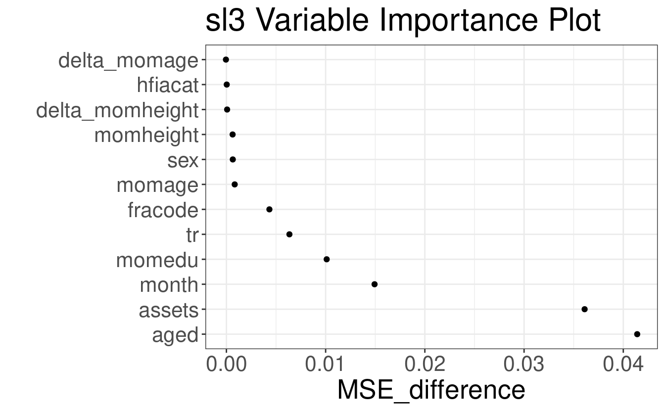
FIGURE 6.2: sl3 variable importance for predicting weight-for-height z-score with WASH Benefits example dataset
According to the sl3 variable importance measures, which were assessed by the
mean squared error (MSE) difference under permutations of each covariate, the
fitted SL’s (sl_fit) most important variables for predicting weight-for-height
z-score (whz) are child age (aged) and household assets (assets) that
reflect the socio-economic status of the study’s subjects.
6.14 Conditional Density Estimation
In certain scenarios it may be useful to estimate the conditional density of a dependent variable, given predictors/covariates that precede it. In the context of causal inference, this arises most readily when working with continuous-valued treatments. Specifically, conditional density estimation (CDE) is necessary when estimating the treatment mechanism for a continuous-valued treatment, often called the generalized propensity score. Compared the classical propensity score (PS) for binary treatments (the conditional probability of receiving the treatment given covariates), \(\mathbb{P}(A = 1 \mid W)\), the generalized PS is the conditional density of treatment \(A\), given covariates \(W\), \(\mathbb{P}(A \mid W)\).
CDE often requires specialized approaches tied to very specific algorithmic
implementations. To our knowledge, general and flexible algorithms for CDE have
been proposed only sparsely in the literature. We have implemented two such
approaches in sl3: a semiparametric CDE approach that makes certain
assumptions about the constancy of (higher) moments of the underlying
distribution, and second approach that exploits the relationship between the
conditional hazard and density functions to allow CDE via pooled hazard
regression. Both approaches are flexible in that they allow the use of arbitrary
regression functions or machine learning algorithms for the estimation of
nuisance quantities (the conditional mean or the conditional hazard,
respectively). We elaborate on these two frameworks below. Importantly, per
Dudoit and van der Laan (2005) and related works, a loss function appropriate for
density estimation is the negative log-density loss \(L(\cdot) = -\log(p_n(\cdot))\).
6.14.1 Moment-restricted location-scale
This family of semiparametric CDE approaches exploits the general form \(\rho(Y - \mu(X) / \sigma(X))\), where \(Y\) is the dependent variable of interest (e.g., treatment \(A\) in the PS), \(X\) are the predictors (e.g., covariates \(W\) in the PS), \(\rho\) is a specified marginal density function, and \(\mu(X) = \E(Y \mid X)\) and \(\sigma(X) = \E[(Y - \mu(X))^2 \mid X]\) are nuisance functions of the dependent variable that may be estimated flexibly. CDE procedures formulated within this framework may be characterized as belonging to a conditional location-scale family, that is, in which \(p_n(Y \mid X) = \rho((Y - \mu_n(X)) / \sigma_n(X))\). While CDE with conditional location-scale families is not without potential disadvantages (e.g., the restriction on the density’s functional form could lead to misspecification bias), this strategy is flexible in that it allows for arbitrary machine learning algorithms to be used in estimating the conditional mean of \(Y\) given \(X\), \(\mu(X) = \E(Y \mid X)\), and the conditional variance of \(Y\) given \(X\), \(\sigma(X) = \E[(Y - \mu(X))^2 \mid X]\).
In settings with limited data, the additional structure imposed by the assumption that the target density belongs to a location-scale family may prove advantageous by smoothing over areas of low support in the data. However, in practice, it is impossible to know whether and when this assumption holds. This procedure is not a novel contribution of our own (and we have been unable to locate a formal description of it in the literature); nevertheless, we provide an informal algorithm sketch below. This algorithm considers access to \(n\) independent and identically distributed (i.i.d.) copies of an observed data random variable \(O = (Y, X)\), an a priori-specified kernel function \(\rho\), a candidate regression procedure \(f_{\mu}\) to estimate \(\mu(X)\), and a candidate regression procedure \(f_{\sigma}\) to estimate \(\sigma(X)\).
- Estimate \(\mu(X) = \E[Y \mid X]\), the conditional mean of \(Y\) given \(X\), by applying the regression estimator \(f_{\mu}\), yielding \(\hat{\mu}(X)\).
- Estimate \(\sigma(X) = \mathbb{V}[Y \mid X]\), the conditional variance of \(Y\) given \(X\), by applying the regression estimator \(f_{\sigma}\), yielding \(\hat{\sigma}^2(X)\). Note that this step involves only estimation of the conditional mean \(\E[(Y - \hat{\mu}(X))^2 \mid X]\).
- Estimate the one-dimensional density of \((Y - \hat{\mu}(X))^2 / \hat{\sigma}^2(X)\), using kernel smoothing to obtain \(\hat{\rho}(Y)\).
- Construct the estimated conditional density \(p_n(Y \mid X) = \hat{\rho}((Y - \hat{\mu}(X)) / \hat{\sigma}(X))\).
This algorithm sketch encompasses two forms of this CDE approach, which diverge
at the second step above. To simplify the approach, one may elect to estimate
only the conditional mean \(\mu(X)\), leaving the conditional variance to be
assumed constant (i.e., estimated simply as the marginal mean of the residuals
\(\E[(Y - \hat{\mu}(X))^2]\)). This subclass of CDE approaches have homoscedastic
error based on the variance assumption made. The conditional variance can
instead by estimated as the conditional mean of the residuals \((Y - \hat{\mu}(X))^2\) given \(X\), \(\E[(Y - \hat{\mu}(X))^2 \mid X]\), where the
candidate algorithm \(f_{\sigma}\) is used to evaluate the expectation. Both
approaches have been implemented in sl3, in the learner
Lrnr_density_semiparametric. The mean_learner argument specifies \(f_{\mu}\)
and the optional var_learner argument specifies \(f_{\sigma}\). We demonstrate
CDE with this approach below.
# semiparametric density estimator with homoscedastic errors (HOSE)
hose_hal_lrnr <- Lrnr_density_semiparametric$new(
  mean_learner = Lrnr_hal9001$new()
)
# semiparametric density estimator with heteroscedastic errors (HESE)
hese_rf_glm_lrnr <- Lrnr_density_semiparametric$new(
  mean_learner = Lrnr_ranger$new()
  var_learner = Lrnr_glm$new()
)

# SL for the conditional treatment density
sl_dens_lrnr <- Lrnr_sl$new(
  learners = list(hose_hal_lrnr, hese_rf_glm_lrnr),
  metalearner = Lrnr_solnp_density$new()
)
6.14.2 Pooled hazard regression
Another approach for CDE available in sl3, and originally proposed in
Dı́az and van der Laan (2011), leverages the relationship between the (conditional) hazard and
density functions. To develop their CDE framework, Dı́az and van der Laan (2011) proposed
discretizing a continuous dependent variable \(Y\) with support \(\mathcal{Y}\)
based on a number of bins \(T\) and a binning procedure (e.g., cutting
\(\mathcal{Y}\) into \(T\) bins of exactly the same length). The tuning parameter
\(T\) conceptually corresponds to the choice of bandwidth in classical kernel
density estimation. Following discretization, each unit is represented by a
collection of records, and the number of records representing a given unit
depends on the rank of the bin (along the discretized support) into which the
unit falls.
To take an example, an instantiation of this procedure might divide the support of \(Y\) into, say, \(T = 4\), bins of equal length (note this requires \(T+1\) cut points): \([\alpha_1, \alpha_2), [\alpha_2, \alpha_3), [\alpha_3, \alpha_4), [\alpha_4, \alpha_5]\) (n.b., the rightmost interval is fully closed while the others are only partially closed). Next, an artificial, repeated measures dataset would be created in which each unit would be represented by up to \(T\) records. To better see this structure, consider an individual unit \(O_i = (Y_i, X_i)\) whose \(Y_i\) value is within \([\alpha_3, \alpha_4)\), the third bin. This unit would be represented by three distinct records: \(\{Y_{ij}, X_{ij}\}_{j=1}^3\), where \(\{\{Y_{ij} = 0\}_{j=1}^2\), \(Y_{i3} = 1\}\) and three exact copies of \(X_i\), \(\{X_{ij}\}_{j=1}^3\). This representation in terms of multiple records for the same unit allows for the conditional hazard probability of \(Y_i\) falling in a given bin along the discretized support to be evaluated via standard binary regression techniques.
In fact, this proposal reformulates the binary regression problem into a corresponding set of hazard regressions: \(\mathbb{P} (Y \in [\alpha_{t-1}, \alpha_t) \mid X) = \mathbb{P} (Y \in [\alpha_{t-1}, \alpha_t) \mid Y \geq \alpha_{t-1}, X) \times \prod_{j = 1}^{t -1} \{1 - \mathbb{P} (Y \in [\alpha_{j-1}, \alpha_j) \mid Y \geq \alpha_{j-1}, X) \}\). Here, the probability of \(Y \in \mathcal{Y}\) falling in bin \([\alpha_{t-1}, \alpha_t)\) may be directly estimated via a binary regression procedure, by re-expressing the corresponding likelihood in terms of the likelihood of a binary variable in a dataset with this repeated measures structure. Finally, the hazard estimates can be mapped into density estimates by re-scaling the hazard estimates by the bin sizes \(\lvert \alpha_t - \alpha_{t-1} \rvert\), that is, \(p_{n, \alpha}(Y \mid X) = \mathbb{P}(Y \in [\alpha_{t-1}, \alpha_t) \mid X) / \lvert \alpha_t - \alpha_{t-1} \rvert\), for \(\alpha_{t-1} \leq a < \alpha_t\). We provide an informal sketch of this algorithm below.
- Apply a procedure to divide the observed support of \(Y\), \(\max(Y) - \min(Y)\), into \(T\) bins: \([\alpha_1, \alpha_2), \ldots, [\alpha_{t-1}, \alpha_t), [\alpha_t, \alpha_{t+1}]\).
- Expand the observed data into a repeated measures data structure, expressing each individual observation as a set of up to \(T\) records, recording the observation ID alongside each such record. For a single unit \(i\), the set of records takes the form \(\{Y_{ij}, X_{ij}\}_{j=1}^{T_i}\), where \(X_{ij}\) are constant in the index set \(\mathcal{J}\), \(Y_{ij}\) is a binary counting process that jumps from \(0\) to \(1\) at its final index (at the bin into which \(Y_i\) falls), and \(T_i \leq T\) indicates the bin along its support into which \(Y_i\) falls.
- Estimate the hazard probability, conditional on \(X\), of bin membership \(\mathbb{P}(Y_i \in [\alpha_{t-1}, \alpha_t) \mid X)\) using any binary regression estimator or appropriate machine learning algorithm.
- Rescale the conditional hazard probability estimates to the conditional density scale by dividing the cumulative hazard by the width of the bin into which \(X_i\) falls, for each observation \(i = 1, \ldots, n\). If the support set is partitioned into bins of equal size (approximately \(n/T\) samples in each bin), this amounts to rescaling by a constant. If the support set is partitioned into bins of equal range, then the rescaling might vary across bins.
A key element of this proposal is the flexibility to use any binary regression
procedure or appropriate machine learning algorithm to estimate \(\mathbb{P}(Y \in [\alpha_{t-1}, \alpha_t) \mid X)\), facilitating the incorporation of
flexibletechniques like ensemble learning (Breiman, 1996; van der Laan et al., 2007).
This extreme degree of flexibility integrates perfectly with the underlying
design principles of sl3; however, we have not yet implemented this approach
in its full generality. A version of this CDE approach, which limits the
original proposal by replacing the use of arbitrary binary regression with the
highly adaptive lasso (HAL) algorithm (Benkeser and van der Laan, 2016) is supported in the
haldensify package
(Hejazi, Benkeser, et al., 2022) (the HAL implementation in haldensify is provided the
hal9001 package (Coyle et al., 2022; Hejazi, Coyle, et al., 2020)). This CDE algorithm that uses haldensify is incorporated
as learner Lrnr_haldensify in sl3, as we demonstrate below.
# learners used for conditional densities for (g_n)
haldensify_lrnr <- Lrnr_haldensify$new(
  n_bins = c(5, 10)
)
Exercises:
Binary outcome prediction
Follow the steps below to predict the probability for myocardial infarction
(mi) using the available covariate data. We thank Dr. David Benkeser,
Assistant Professor of Biostatistics and Bioinformatics at Emory University, for
making this Cardiovascular Health Study (CHS) publicly data available.
# load the data set
library(readr)
db_data <- url(
  paste0(
    "https://raw.githubusercontent.com/benkeser/sllecture/master/",
    "chspred.csv"
  )
)
chspred <- read_csv(file = db_data, col_names = TRUE)
Let’s take a quick peek at the data:
head(chspred)| waist | alcoh | hdl | beta | smoke | ace | ldl | bmi | aspirin | gend | age | estrgn | glu | ins | cysgfr | dm | fetuina | whr | hsed | race | logcystat | logtrig | logcrp | logcre | health | logkcal | sysbp | mi |
|---|---|---|---|---|---|---|---|---|---|---|---|---|---|---|---|---|---|---|---|---|---|---|---|---|---|---|---|
| 110.16 | 0.000 | 66.50 | 0 | 0 | 1 | 114.2 | 28.00 | 0 | 0 | 73.52 | 0 | 159.93 | 70.334 | 75.01 | 1 | 0.1752 | 1.1690 | 1 | 1 | -0.3420 | 5.406 | 2.0126 | -0.6739 | 0 | 4.393 | 177.13 | 0 |
| 89.98 | 0.000 | 50.07 | 0 | 0 | 0 | 103.8 | 20.89 | 0 | 0 | 61.77 | 0 | 153.39 | 33.969 | 82.74 | 1 | 0.5717 | 0.9011 | 0 | 0 | -0.0847 | 4.859 | 3.2933 | -0.5551 | 1 | 6.207 | 136.37 | 0 |
| 106.19 | 8.417 | 40.51 | 0 | 0 | 0 | 165.7 | 28.46 | 1 | 1 | 72.93 | 0 | 121.71 | -17.302 | 74.70 | 0 | 0.3517 | 1.1797 | 0 | 1 | -0.4451 | 4.509 | 0.3013 | -0.0115 | 0 | 6.732 | 135.20 | 0 |
| 90.06 | 0.000 | 36.17 | 0 | 0 | 0 | 45.2 | 23.96 | 0 | 0 | 79.12 | 0 | 53.97 | 11.732 | 95.78 | 0 | 0.5439 | 1.1360 | 0 | 0 | -0.4807 | 5.183 | 3.0243 | -0.5751 | 1 | 7.397 | 139.02 | 0 |
| 78.61 | 2.979 | 71.06 | 0 | 1 | 0 | 131.3 | 10.97 | 0 | 1 | 69.02 | 0 | 94.32 | 9.711 | 72.71 | 0 | 0.4916 | 1.1028 | 1 | 0 | 0.3121 | 4.219 | -0.7057 | 0.0053 | 1 | 8.278 | 88.05 | 0 |
| 91.66 | 0.000 | 59.50 | 0 | 0 | 0 | 171.2 | 29.13 | 0 | 1 | 81.83 | 0 | 212.91 | -28.227 | 69.22 | 1 | 0.4621 | 0.9529 | 1 | 0 | -0.2872 | 5.177 | 0.9705 | 0.2127 | 1 | 5.994 | 69.59 | 0 |
- Create an
sl3task, setting myocardial infarctionmias the outcome and using all available covariate data. - Make a library of seven relatively fast base learning algorithms (i.e., do not consider BART or HAL). Customize tuning parameters for one of your learners. Incorporate at least one screener-learner coupling.
- Make the SL and train it on the task.
- Print the SL fit results by adding
$cv_risk(loss_squared_error)to your fit object.
6.15 Concluding Remarks
Super Learner (SL) is a general approach that can be applied to a diversity of estimation and prediction problems which can be defined by a loss function.
-
It would be straightforward to plug in the estimator returned by SL into the target parameter mapping.
- For example, suppose we are after the average treatment effect (ATE) of a binary treatment intervention: \(\Psi_0 = E_{0,W}[E_0(Y|A=1,W) - E_0(Y|A=0,W)]\).
- We could use the SL that was trained on the original data (let’s call
this
sl_fit) to predict the outcome for all subjects under each intervention. All we would need to do is take the average difference between the counterfactual outcomes under each intervention of interest. - Considering \(\Psi_0\) above, we would first need two \(n\)-length vectors of predicted outcomes under each intervention. One vector would represent the predicted outcomes under an intervention that sets all subjects to receive \(A=1\), \(Y_i|A_i=1,W_i\) for all \(i=1,\ldots,n\). The other vector would represent the predicted outcomes under an intervention that sets all subjects to receive \(A=0\), \(Y_i|A_i=0,W_i\) for all \(i=1,\ldots,n\).
- After obtaining these vectors of counterfactual predicted outcomes, all we would need to do is average and then take the difference in order to “plug-in” the SL estimator into the target parameter mapping.
- In
sl3and with our current ATE example, this could be achieved withmean(sl_fit$predict(A1_task)) - mean(sl_fit$predict(A0_task)); whereA1_task$datawould contain all 1’s (or the level that pertains to receiving the treatment) for the treatment column in the data (keeping all else the same), andA0_task$datawould contain all 0’s (or the level that pertains to not receiving the treatment) for the treatment column in the data.
It’s a worthwhile exercise to obtain the predicted counterfactual outcomes and create these counterfactual
sl3tasks. It’s too biased, however, to plug the SL fit into the target parameter mapping, (e.g., calling the result ofmean(sl_fit$predict(A1_task)) - mean(sl_fit$predict(A0_task))the estimated ATE. We would end up with an estimator for the ATE that was optimized for estimation of the prediction function, and not the ATE!-
Ultimately, we want an estimator that is does the best job in approximating our question of interest. That is, we care about doing a the best job possible estimating \(\psi_0\). The SL is an essential step to help us get there: the counterfactual predicted outcome estimates (like those explained above), and other SL-derived estimates (like a propensity score) play a key role in estimating \(\psi_0\). However, SL is not the end of the estimation procedure. Specifically, if we simply plugged in the SL estimates into the target parameter, we would not have an asymptotically linear estimator of the target estimand; the SL is not an efficient substitution estimator and does not admit statistical inference. Why does this matter?
An asymptotically linear estimator is one that converges to the estimand a \(\frac{1}{\sqrt{n}}\) rate, thereby permitting formal statistical inference, i.e., confidence intervals and \(p\)-values, (see Chapters 4–6 of van der Laan and Rose (2011)).
Substitution, or plug-in, estimators are desirable because they respect both the local and global constraints of the statistical model, such as bounds on an outcome, and have they have better finite-sample properties (see Chapter 6 of van der Laan and Rose (2011)).
-
An efficient estimator is optimal in the sense that it has the lowest possible variance, and is thus the most precise. An estimator is efficient if and only if is asymptotically linear with influence curve equal to the canonical gradient (see Chapter 6 of van der Laan and Rose (2011)).
- The canonical gradient is a mathematical object that is specific to the target estimand, and it provides information on the level of difficulty of the estimation problem (Chapter 5 of van der Laan and Rose (2011)). Various canonical gradients are shown in the chapters that follow.
- Practitioners do not need to know how to calculate a canonical gradient to explain properties that are desirable for an estimator to possess (like substitution/plug-in, admits valid inference, efficient, and ability to optimize finite sample performance). These properties motivate the use TMLE, since TMLE satisfies them.
TMLE is a general strategy that succeeds in constructing efficient and asymptotically linear plug-in estimators that are robust in finite samples.
SL is fantastic for pure prediction, and for obtaining initial estimates of components in the likelihood (the first step of TMLE), but we need the second, targeting/updating/fluctuation, step to have the desirable statistical properties mentioned above.
In the chapters that follow, we focus on various targeted maximum likelihood estimator and the targeted minimum loss-based estimator, both referred to as TMLE.
6.16 Appendix
6.16.1 Exercise 1 Solution
Here is a potential solution to the sl3 Exercise 1 – Predicting Myocardial
Infarction with
sl3.
db_data <- url(
  "https://raw.githubusercontent.com/benkeser/sllecture/master/chspred.csv"
)
chspred <- read_csv(file = db_data, col_names = TRUE)
data.table::setDT(chspred)

# make task
chspred_task <- make_sl3_Task(
  data = chspred,
  covariates = colnames(chspred)[-1],
  outcome = "mi"
)

# make learners
glm_learner <- Lrnr_glm$new()
lasso_learner <- Lrnr_glmnet$new(alpha = 1)
ridge_learner <- Lrnr_glmnet$new(alpha = 0)
enet_learner <- Lrnr_glmnet$new(alpha = 0.5)
# curated_glm_learner uses formula = "mi ~ smoke + beta"
curated_glm_learner <- Lrnr_glm_fast$new(covariates = c("smoke", "beta"))
mean_learner <- Lrnr_mean$new() # That is one mean learner!
glm_fast_learner <- Lrnr_glm_fast$new()
ranger_learner <- Lrnr_ranger$new()
svm_learner <- Lrnr_svm$new()
xgb_learner <- Lrnr_xgboost$new()

# screening
screen_cor <- make_learner(Lrnr_screener_correlation)
glm_pipeline <- make_learner(Pipeline, screen_cor, glm_learner)

# stack learners together
stack <- make_learner(
  Stack,
  glm_pipeline, glm_learner,
  lasso_learner, ridge_learner, enet_learner,
  curated_glm_learner, mean_learner, glm_fast_learner,
  ranger_learner, svm_learner, xgb_learner
)

# make and train SL
sl <- Lrnr_sl$new(
  learners = stack
)
sl_fit <- sl$train(chspred_task)
sl_fit$cv_risk(loss_squared_error)