8 Dynamic and Optimal Individualized Treatment Regimes

Ivana Malenica

Based on the tmle3mopttx R package by Ivana Malenica, Jeremy Coyle, and Mark van der Laan.

8.1 Learning Objectives

Differentiate dynamic and optimal dynamic treatment interventions from static interventions.
Explain the benefits, and challenges, associated with using optimal individualized treatment regimes in practice.
Contrast the impact of implementing an optimal individualized treatment regime in the population with the impact of implementing static and dynamic treatment regimes in the population.
Estimate causal effects under optimal individualized treatment regimes with the tmle3mopttx R package.
Assess the mean under optimal individualized treatment with resource constraints.
Implement optimal individualized treatment rules based on sub-optimal rules, or “simple” rules, and recognize the practical benefit of these rules.
Construct “realistic” optimal individualized treatment regimes that respect real data and subject-matter knowledge limitations on interventions by only considering interventions that are supported by the data.
Interpret the estimated optimal individualized treatment rule.
Measure variable importance as defined in terms of the optimal individualized treatment interventions.

8.2 Introduction to Optimal Individualized Interventions

Identifying which intervention will be effective for which patient based on lifestyle, genetic and environmental factors is a common goal in precision medicine. To put it in context, Abacavir and Tenofovir are commonly prescribed as part of the antiretroviral therapy to Human Immunodeficiency Virus (HIV) patients. However, not all individuals benefit from the two medications equally. In particular, patients with renal dysfunction might further deteriorate if prescribed Tenofovir, due to the high nephrotoxicity caused by the medication. While Tenofovir is still highly effective treatment option for HIV patients, in order to maximize the patient’s well-being, it would be beneficial to prescribe Tenofovir only to individuals with healthy kidney function. As an another example, consider a HIV trial where our goal is to improve retention in HIV care. In a randomized clinical trial, several interventions show efficacy- including appointment reminders through text messages, small cash incentives for on time clinic visits, and peer health workers. Ideally, we want to improve effectiveness by assigning each patient the intervention they are most likely to benefit from, as well as improve efficiency by not allocating resources to individuals that do not need them, or would not benefit from it.

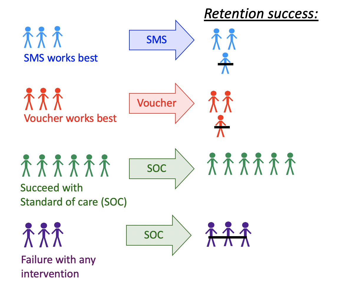
FIGURE 5.1: Dynamic Treatment Regime in a Clinical Setting

One opts to administer the intervention to individuals who will profit from it, instead of assigning treatment on a population level. But how do we know which intervention works for which patient? This aim motivates a different type of intervention, as opposed to the static exposures we described in previous chapters. In particular, in this chapter we learn about dynamic or “individualized” interventions that tailor the treatment decision based on the collected covariates. Formally, dynamic treatments represent interventions that at each treatment-decision stage are allowed to respond to the currently available treatment and covariate history. A dynamic treatment rule can be thought of as a rule where the input is the available set of collected covariates, and the output is an individualized treatment for each patient (Bembom and van der Laan, 2007; Chakraborty and Moodie, 2013; J Robins, 1986).

In the statistics community such a treatment strategy is termed an individualized treatment regime (ITR), also known as the optimal dynamic treatment rule, optimal treatment regime, optimal strategy, and optimal policy (Murphy, 2003; Robins, 2004). The (counterfactual) population mean outcome under an ITR is the value of the ITR (Murphy, 2003; Robins, 2004). Even more, suppose one wishes to maximize the population mean of an outcome, where for each individual we have access to some set of measured covariates. This means, for example, that we can learn for which individual characteristics assigning treatment increases the probability of a beneficial outcome. An ITR with the maximal value is referred to as an optimal ITR or the optimal individualized treatment. Consequently, the value of an optimal ITR is termed the optimal value, or the mean under the optimal individualized treatment.

The problem of estimating the optimal individualized treatment has received much attention in the statistics literature over the years, especially with the advancement of precision medicine; see Murphy (2003), Robins (2004), Zhang et al. (2016), Zhao et al. (2012), Chakraborty and Moodie (2013) and Robins and Rotnitzky (2014) to name a few. However, much of the early work depends on parametric assumptions. As such, even in a randomized trial, the statistical inference for the optimal individualized treatment relies on assumptions that are generally believed to be false, and can lead to biased results.

In this chapter, we consider estimation of the mean outcome under the optimal individualized treatment where the candidate rules are restricted to depend only on user-supplied subset of the baseline covariates. The estimation problem is addressed in a statistical model for the data distribution that is nonparametric, and at most places restrictions on the probability of a patient receiving treatment given covariates (as in a randomized trial). As such, we don’t need to make any assumptions about the relationship of the outcome with the treatment and covariates, or the relationship between the treatment and covariates. Further, we provide a Targeted Maximum Likelihood Estimator for the mean under the optimal individualized treatment that allows us to generate valid inference for our parameter, without having any parametric assumptions.

In the following, we provide a brief overview of the methodology with a focus on building intuition for the target parameter and its importance — aided with simulations, data examples and software demonstrations. For more information on the technical aspects of the algorithm, further practical advice and overview, the interested reader is invited to additionally consult van der Laan and Luedtke (2015), A Luedtke and van der Laan (2016), Montoya, van der Laan, Luedtke, et al. (2023) and Montoya, van der Laan, Skeem, et al. (2023).

8.3 Data Structure and Notation

Suppose we observe \(n\) independent and identically distributed observations of the form \(O=(W,A,Y) \sim P_0\). We denote \(A\) as categorical treatment, and \(Y\) as the final outcome. In particular, we define \(A \in \mathcal{A}\) where \(\mathcal{A} \equiv \{a_1, \cdots, a_{n_A} \}\) and \(n_A = |\mathcal{A}|\), with \(n_A\) denoting the number of categories (possibly only two, for a binary setup). Note that we treat \(W\) as vector-valued, representing all of our collected baseline covariates. Therefore, for a single random individual \(i\), we have that their observed data is \(O_i\): with corresponding baseline covariates \(W_i\), treatment \(A_i\), and final outcome \(Y_i\). Let \(O^n = \{O_i\}_{i=1}^n\) denote \(n\) observed samples. Then, we say that \(O^n \sim P_0\), or that all data was drawn from some true probability distribution \(P_0\). Let \(\mathcal{M}\) denote a statistical model for the probability distribution of the data that is nonparametric, beyond possible knowledge of the treatment mechanism. In words, this means that we make no assumptions on the relationship between variables, but might be able to say something about the relationship of \(A\) and \(W\), as is the case in a randomized trial. In general, the more we know, or are willing to assume about the experiment that produces the data, the smaller the model. The true data generating distribution \(P_0\) is part of the statistical model \(\mathcal{M}\), and we write \(P_0 \in \mathcal{M}\). As in previous chapters, we denote \(P_n\) as the empirical distribution which gives each observation weight \(1/n\).

We use the structural equation model (SEM) in order to define the process that gives rise to the observed (endogenous) and not observed (exogenous) variables, as described by Pearl (2009). In particular, we denote \(U=(U_W,U_A,U_Y)\) as the exogenous random variables, drawn from \(U \sim P_U\). The endogenous variables, written as \(O=(W,A,Y)\), correspond to the observed data. We can define the relationships between variables with the following structural equations: \[\begin{align} W &= f_W(U_W) \\ A &= f_A(W, U_A) \\ Y &= f_Y(A, W, U_Y), \tag{8.1} \end{align}\] where the collection \(f=(f_W,f_A,f_Y)\) denotes unspecified functions, beyond possible knowledge of the treatment mechanism function, \(f_A\). Note that in the case of a randomized trial, we can write the above NPSEM as \[\begin{align} W &= f_W(U_W) \\ A &= U_A \\ Y &= f_Y(A, W, U_Y), \tag{8.2} \end{align}\] where \(U_A\) has a known distribution and \(U_A\) is independent of \(U_W\). We will discuss this more in later sections on identifiability.

The likelihood of the data admits a factorization, implied by the time ordering of \(O\). We denote the true density of \(O\) as \(p_0\), corresponding to the distribution \(P_0\) and dominating measure \(\mu\). \[\begin{equation} p_0(O) = p_{Y,0}(Y \mid A,W) p_{A,0}(A \mid W) p_{W,0}(W) = q_{Y,0}(Y \mid A,W) g_{A,0}(A \mid W) q_{W,0}(W), \tag{8.3} \end{equation}\] where \(p_{Y,0}(Y|A,W)\) is the conditional density of \(Y\) given \((A, W)\) with respect to some dominating measure \(\mu_Y\), \(p_{A,0}\) is the conditional density of \(A\) given \(W\) with respect to a counting measure \(\mu_A\), and \(p_{W,0}\) is the density of \(W\) with respect to dominating measure \(\mu_W\). In order to match relevant Targeted Learning literature, we also write \(P_{Y,0}(Y \mid A, W) = Q_{Y,0}(Y \mid A,W)\), \(P_{A,0}(A \mid W) = g_0(A \mid W)\) and \(P_{W,0}(W)=Q_{W,0}(W)\) as the corresponding conditional distribution of \(Y\) given \((A,W)\), treatment mechanism \(A\) given \(W\), and distribution of baseline covariates. For notational simplicity, we additionally define \(\bar{Q}_{Y,0}(A,W) \equiv \E_0[Y \mid A,W]\) as the conditional expectation of \(Y\) given \((A,W)\).

Lastly, we define \(V\) as a subset of the baseline covariates the optimal individualized rule depends on, where \(V \in W\). Note that \(V\) could be all of \(W\), or an empty set, depending on the subject matter knowledge. In particular, a researcher might want to consider known effect modifiers available at the time of treatment decision as possible \(V\) covariates, or consider dynamic treatment rules based on measurments that can be easily obtained in a clinical setting. Defining \(V\) as a more restrictive set of baseline covariates allows us to consider possibly sub-optimal rules that are easier to estimate, and thereby allows for statistical inference for the counterfactual mean outcome under the sub-optimal rule; we will elaborate on this in later sections.

8.4 Defining the Causal Effect of an Optimal Individualized Intervention

Consider dynamic treatment rules, denoted as \(d\), in the set of all possible rules \(\mathcal{D}\). Then, in a point treatment setting, \(d\) is a deterministic function that takes as input \(V\) and outputs a treatment decision where \(V \rightarrow d(V) \in \{a_1, \cdots, a_{n_A} \}\). We will use dynamic treatment rules, and the corresponding treatment decision, to describe an intervention on the treatment mechanism and the corresponding outcome under a dynamic treatment rule.

As mentioned in the previous section, causal effects are defined in terms of hypothetical interventions on the SEM (8.1). For a given rule \(d\), our modified system then takes the following form: \[\begin{align} W &= f_W(U_W) \\ A &= d(V) \\ Y_{d(V)} &= f_Y(d(V), W, U_Y), \tag{8.4} \end{align}\] where the dynamic treatment regime may be viewed as an intervention in which \(A\) is set equal to a value based on a hypothetical regime \(d(V)\). The couterfactual outcome \(Y_{d(V)}\) denotes the outcome for a patient had their treatment been assigned using the dynamic rule \(d(V)\), possibly contrary to the fact. Similarly, the counterfactual outcomes had all patients been assigned treatment (\(A=1\)), or given control (\(A=0\)), are written as \(Y_1\) and \(Y_0\). Finally, we denote the distribution of the counterfactual outcomes as \(P_{U,X}\), implied by the distribution of exogenous variables \(U\) and structural equations \(f\). The set of all possible counterfactual distributions are encompased by the causal model \(\mathcal{M}^F\), where \(P_{U,X} \in \mathcal{M}^F\).

The goal of any causal analysis motivated by such dynamic interventions is to estimate a parameter defined as the counterfactual mean of the outcome with respect to the modified intervention distribution. That is, subject’s outcome if, possibly contrary to the fact, the subject received treatment that would have been assigned by rule \(d(V)\). Equivalently, we ask the following causal question: “What is the expected outcome had every subject received treatment according to the (optimal) individualized treatment?” In order to estimate the optimal individualized treatment, we set the following optimization problem:

\[d_{opt}(V) \equiv \text{argmax}_{d(V) \in \mathcal{D}} \E_{P_{U,X}}[Y_{d(V)}], \] where the optimal individualized rule is the rule with the maximal value. We note that, in case the problem at hand requires minimizing the mean of an outcome, our optimal individualized rule will be the rule with the minimal value instead.

With that in mind, we can consider different treatment rules, all in the set \(\mathcal{D}\):

The true rule, \(d_{0,\text{opt}}\), and the corresponding causal parameter \(\E_{U,X}[Y_{d_{0,\text{opt}}(V)}]\) denoting the expected outcome under the true optimal treatment rule \(d_{0,\text{opt}}(V)\).
The estimated rule, \(d_{n,\text{opt}}\), and the corresponding causal parameter \(\E_{U,X}[Y_{d_{n,\text{opt}}(V)}]\) denoting the expected outcome under the estimated optimal treatment rule \(d_{n,\text{opt}}(V)\).

In this chapter, we will focus on the value under the estimated optimal rule \(d_{n,\text{opt}}\), a data-adaptive parameter. Note that its true value depends on the sample! Finally, our causal target parameter of interest is the expected outcome under the estimated optimal individualized rule:

\[\Psi_{d_{n, \text{opt}}(V)}(P_{U,X}) \coloneqq \E_{P_{U,X}}[Y_{d_{n, \text{opt}}(V)}].\]

8.4.1 Identification and Statistical Estimand

The optimal individualized rule, as well as the value of an optimal individualized rule, are causal parameters based on the unobserved counterfactuals. In order for the causal quantities to be estimated from the observed data, they need to be identified with statistical parameters. This step of the roadmap requires we make a few assumptions:

Strong ignorability: \(A \indep Y^{d_{n, \text{opt}}(v)} \mid W\), for all \(a \in \mathcal{A}\).
Positivity (or overlap): \(P_0(\min_{a \in \mathcal{A}} g_0(a \mid W) > 0) = 1\)

Under the above assumptions, we can identify the causal target parameter with observed data using the G-computation formula. The value of an individualized rule can now be expressed as

\[\E_0[Y_{d_{n, \text{opt}}(V)}] = \E_{0,W}[\bar{Q}_{Y,0}(A=d_{n, \text{opt}}(V),W)],\]

which, under assumptions, is interpreted as the mean outcome if (possibly contrary to fact), treatment was assigned according to the optimal rule. Finally, the statistical counterpart to the causal parameter of interest is defined as

\[\psi_0 = \E_{0,W}[\bar{Q}_{Y,0}(A=d_{n,\text{opt}}(V),W)].\]

Inference for the optimal value has been shown to be difficult at exceptional laws, defined as probability distributions for which there is a positive probability on a set of \(W\) values for which conditional expectation of \(Y\) given \(A\) and \(W\) is constant in \(a\) - so all treatments are equally benefitial. Inference is similarly difficult in finite samples if the treatment effect is very small in all strata, even though valid asymptotic estimators exist in this setting. With that in mind, we address the estimation problem under the assumption of non-exceptional laws in effect.

Many methods for learning the optimal rule from data have been developed (Chakraborty and Moodie, 2013; Murphy, 2003; Robins, 2004; Zhang et al., 2016; Zhao et al., 2012). In this chapter, we focus on the methods discussed in A Luedtke and van der Laan (2016) and van der Laan and Luedtke (2015). Note however, that tmle3mopttx also supports the widely used Q-learning approach, where the optimal individualized rule is based on the initial estimate of \(\bar{Q}_{Y,0}(A,W)\) (Sutton et al., 1998).

We follow the methodology outlined in A Luedtke and van der Laan (2016) and van der Laan and Luedtke (2015), where we learn the optimal ITR using Super Learner (van der Laan et al., 2007), and estimate its value with cross-validated Targeted Minimum Loss-based Estimation (CV-TMLE) (Zheng and van der Laan, 2011). In great generality, we first need to estimate the true individual treatment regime, \(d_0(V)\), which corresponds to dynamic treatment rule that takes a subset of covariates \(V\) and assigns treatment to each individual based on their observed covariates \(v\). With the estimate of the true optimal ITR in hand, we can estimate its corresponding value.

8.4.2 Binary treatment

How do we estimate the optimal individualized treatment regime? In the case of a binary treatment, a key quantity for optimal ITR is the blip function. One can show that any optimal ITR assigns treatment to individuals falling in strata in which the stratum specific average treatment effect, the blip, is positive and does not assign treatment to individuals for which this quantity is negative. Therefore for a binary treatment, under causal assumptions, we define the blip function as: \[\bar{Q}_0(V) \equiv \E_0[Y_1-Y_0 \mid V] \equiv \E_0[\bar{Q}_{Y,0}(1,W) - \bar{Q}_{Y,0}(0,W) \mid V],\] or the average treatment effect within a stratum of \(V\). The note that the optimal individualized rule can now be derived as \(d_{n,\text{opt}}(V) = \mathbb{I}(\bar{Q}_{n}(V) > 0)\).

The package tmle3mopttx relies on using the Super Learner to estimate the blip function. With that in mind, the loss function utilized for learning the optimal individualized rule corresponds to conditional mean type losses. It is however worth mentioning that A Luedtke and van der Laan (2016) present three different approaches for learning the optimal rule. Namely, they focus on:

Super Learner of the blip function using the squared error loss,
Super Learner of \(d_0\) using the weighted classification loss function,
Super Learner of \(d_0\) that uses a library of candidate estimators that are implied by estimators of the blip as well as estimators that directly go for \(d_0\) through weighted classification.

A benefit of relying on the blip function, as implemented in tmle3mopttx, is that one can look at the distribution of the predicted outcomes of the blip for a given sample. Having an estimate of the blip allows one to identify patients in the sample who benefit the most (or the least) from treatment. Additionally, blip-based approach allows for straight-forward extension to the categorical treatment, interpretable rules, and OIT under resource constrains, where only a percent of the population can receive treatment (AR Luedtke and van der Laan, 2016).

Relying on the Targeted Maximum Likelihood (TML) estimator and the Super Learner estimate of the blip function, we follow the below steps in order to obtain value of the ITR:

Estimate \(\bar{Q}_{Y,0}(A,W)\) and \(g_0(A \mid W)\) using sl3. We denote such estimates as \(\bar{Q}_{Y,n}(A,W)\) and \(g_n(A \mid W)\).
Apply the doubly robust Augmented-Inverse Probability Weighted (A-IPW) transform to our outcome (double-robust pseudo-outcome), where we define: \[D_{\bar{Q}_Y,g,a}(O) \equiv \frac{\mathbb{I}(A=a)}{g(A \mid W)} (Y - \bar{Q}_Y(A,W)) + \bar{Q}_Y(A=a,W).\]

Note that under the randomization and positivity assumptions we have that \(\E[D_{\bar{Q}_Y,g,a}(O) \mid V] = \E[Y_a \mid V]\). We emphasize the double robust nature of the A-IPW transform — consistency of \(\E[Y_a \mid V]\) will depend on correct estimation of either \(\bar{Q}_{Y,0}(A,W)\) or \(g_0(A \mid W)\). As such, in a randomized trial, we are guaranteed a consistent estimate of \(\E[Y_a \mid V]\) even if we get \(\bar{Q}_{Y,0}(A,W)\) wrong! An alternative to the double-robust pseudo-outcome just presented would be single stage Q-learning, where an estimate \(\bar{Q}_{Y,0}(A,W)\) is used to predict at \(\bar{Q}_{Y,n}(A=1,W)\) and \(\bar{Q}_{Y,n}(A=0,W)\). This provides an estimate of the blip function, \(\bar{Q}_{Y,n}(A=1,W) - \bar{Q}_{Y,n}(A=0,W)\), but relies on doing a good job on estimating \(\bar{Q}_{Y,0}(A,W)\).

Using the double-robust pseudo-outcome, we can define the following contrast: \[D_{\bar{Q}_Y,g}(O) = D_{\bar{Q}_Y, g, a=1}(O) - D_{\bar{Q}_Y, g, a=0}(O).\]

We estimate the blip function, \(\bar{Q}_{0,a}(V)\), by regressing \(D_{\bar{Q}_Y,g}(O)\) on \(V\) using the specified sl3 library of learners and an appropriate loss function. Finally, we are ready for the final steps.

Our estimated rule corresponds to \(\text{argmax}_{a \in \mathcal{A}} \bar{Q}_{0,a}(V)\).
We obtain inference for the mean outcome under the estimated optimal rule using CV-TMLE.

8.4.3 Categorical treatment

In line with the approach considered for binary treatment, we extend the blip function to allow for categorical treatment. We denote such blip function extensions as pseudo-blips, which are our new estimation targets in a categorical setting. We define pseudo-blips as vector-valued entities where the output for a given \(V\) is a vector of length equal to the number of treatment categories, \(n_A\). As such, we define it as: \[\bar{Q}_0^{pblip}(V) = \{\bar{Q}_{0,a}^{pblip}(V): a \in \mathcal{A} \}\]

We implement three different pseudo-blips in tmle3mopttx.

Blip1 corresponds to choosing a reference category of treatment, and defining the blip for all other categories relative to the specified reference. Hence we have that: \[\bar{Q}_{0,a}^{pblip-ref}(V) \equiv \E_0[Y_a-Y_0 \mid V]\] where \(Y_0\) is the specified reference category with \(A=0\). Note that, for the case of binary treatment, this strategy reduces to the approach described for the binary setup.
Blip2 approach corresponds to defining the blip relative to the average of all categories. As such, we can define \(\bar{Q}_{0,a}^{pblip-avg}(V)\) as: \[\bar{Q}_{0,a}^{pblip-avg}(V) \equiv \E_0 [Y_a - \frac{1}{n_A} \sum_{a \in \mathcal{A}} Y_a \mid V].\] In the case where subject-matter knowledge regarding which reference category to use is not available, blip2 might be a viable option.
Blip3 reflects an extension of Blip2, where the average is now a weighted average: \[\bar{Q}_{0,a}^{pblip-wavg}(V) \equiv \E_0 [ Y_a - \frac{1}{n_A} \sum_{a \in \mathcal{A}} Y_{a} P(A=a \mid V) \mid V ].\]

Just like in the binary case, pseudo-blips are estimated by regressing contrasts composed using the A-IPW transform on \(V\).

8.4.4 Technical Note: Inference and data-adaptive parameter

In a randomized trial, statistical inference relies on the second-order difference between the estimate of the optimal individualized treatment and the optimal individualized treatment itself to be asymptotically negligible. This is a reasonable condition if we consider rules that depend on a small number of covariates, or if we are willing to make smoothness assumptions. Alternatively, we can consider TMLEs and statistical inference for data-adaptive target parameters defined in terms of an estimate of the optimal individualized treatment. In particular, instead of trying to estimate the mean under the true optimal individualized treatment, we aim to estimate the mean under the estimated optimal individualized treatment. As such, we develop cross-validated TMLE approach that provides asymptotic inference under minimal conditions for the mean under the estimate of the optimal individualized treatment. In particular, considering the data adaptive parameter allows us to avoid consistency and rate condition for the fitted optimal rule, as required for asymptotic linearity of the TMLE of the mean under the actual, true optimal rule. Practically, the estimated (data-adaptive) rule should be preferred, as this possibly sub-optimal rule is the one implemented in the population.

8.4.5 Technical Note: Why CV-TMLE?

As discussed in van der Laan and Luedtke (2015), CV-TMLE is necessary as the non-cross-validated TMLE is biased upward for the mean outcome under the rule, and therefore overly optimistic. More generally however, using CV-TMLE allows us more freedom in estimation and therefore greater data adaptivity, without sacrificing inference.

8.5 Interpreting the Causal Effect of an Optimal Individualized Intervention

In summary, the mean outcome under the optimal individualized treatment is a counterfactual quantity of interest representing what the mean outcome would have been if everybody, contrary to the fact, received treatment that optimized their outcome. The optimal individualized treatment regime is a rule that optimizes the mean outcome under the dynamic treatment, where the candidate rules are restricted to only respond to a user-supplied subset of the baseline covariates. In essence, our target parameter answers the key aim of precision medicine: allocating the available treatment by tailoring it to the individual characteristics of the patient, with the goal of optimizing the final outcome.

8.6 Evaluating the Causal Effect of an OIT with Binary Treatment

Finally, we demonstrate how to evaluate the mean outcome under the optimal individualized treatment using tmle3mopptx. To start, let’s load the packages we’ll use and set a seed:

library(data.table)
library(sl3)
library(tmle3)
library(tmle3mopttx)
library(devtools)

set.seed(111)

8.6.1 Simulated Data

First, we load the simulated data. We will start with the more general setup where the treatment is a binary variable; later in the chapter we will consider another data-generating distribution where \(A\) is categorical. In this example, our data generating distribution is of the following form: \[\begin{align*} W &\sim \mathcal{N}(\bf{0},I_{3 \times 3})\\ \P(A=1 \mid W) &= \frac{1}{1+\exp^{(-0.8*W_1)}}\\ \P(Y=1 \mid A,W) &= 0.5\text{logit}^{-1}[-5I(A=1)(W_1-0.5)+5I(A=0)(W_1-0.5)] + 0.5\text{logit}^{-1}(W_2W_3) \end{align*}\]

data("data_bin")

The above composes our observed data structure \(O = (W, A, Y)\). Note that the truth is \(\psi=0.578\) for this data generating distribution.

To formally express this fact using the tlverse grammar introduced by the tmle3 package, we create a single data object and specify the functional relationships between the nodes in the directed acyclic graph (DAG) via structural equation models (SEMs), reflected in the node list that we set up:

# organize data and nodes for tmle3
data <- data_bin
node_list <- list(
  W = c("W1", "W2", "W3"),
  A = "A",
  Y = "Y"
)

We now have an observed data structure (data) and a specification of the role that each variable in the dataset plays as the nodes in a DAG.

8.6.2 Constructing Optimal Stacked Regressions with `sl3`

To easily incorporate ensemble machine learning into the estimation procedure, we rely on the facilities provided in the sl3 R package. Using the framework provided by the sl3 package, the nuisance parameters of the TML estimator may be fit with ensemble learning, using the cross-validation framework of the Super Learner algorithm of van der Laan et al. (2007).

# Define sl3 library and metalearners:
lrn_xgboost_50 <- Lrnr_xgboost$new(nrounds = 50)
lrn_xgboost_100 <- Lrnr_xgboost$new(nrounds = 100)
lrn_xgboost_500 <- Lrnr_xgboost$new(nrounds = 500)

lrn_mean <- Lrnr_mean$new()
lrn_glm <- Lrnr_glm_fast$new()
lrn_lasso <- Lrnr_glmnet$new()

## Define the Q learner:
Q_learner <- Lrnr_sl$new(
  learners = list(lrn_lasso, lrn_mean, lrn_glm),
  metalearner = Lrnr_nnls$new()
)

## Define the g learner:
g_learner <- Lrnr_sl$new(
  learners = list(lrn_lasso, lrn_glm),
  metalearner = Lrnr_nnls$new()
)

## Define the B learner:
b_learner <- Lrnr_sl$new(
  learners = list(lrn_lasso,lrn_mean, lrn_glm),
  metalearner = Lrnr_nnls$new()
)

As seen above, we generate three different ensemble learners that must be fit, corresponding to the learners for the outcome regression (Q), propensity score (g), and the blip function (B). We make the above explicit with respect to standard notation by bundling the ensemble learners into a list object below:

# specify outcome and treatment regressions and create learner list
learner_list <- list(Y = Q_learner, A = g_learner, B = b_learner)

The learner_list object above specifies the role that each of the ensemble learners we’ve generated is to play in computing initial estimators. Recall that we need initial estimators of relevant parts of the likelihood in order to build a TMLE for the parameter of interest. In particular, learner_list makes explicit the fact that our Y is used in fitting the outcome regression, while A is used in fitting the treatment mechanism regression, and finally B is used in fitting the blip function.

8.6.3 Targeted Estimation of the Mean under the Optimal Individualized Interventions Effects

To start, we will initialize a specification for the TMLE of our parameter of interest simply by calling tmle3_mopttx_blip_revere. We specify the argument V = c("W1", "W2", "W3") when initializing the tmle3_Spec object in order to communicate that we’re interested in learning a rule dependent on V covariates. Note that we don’t have to specify V — this will result in a rule that is not based on any collected covariates; we will see an example like this shortly. We also need to specify the type of (pseudo) blip we will use in this estimation problem, the list of learners used to estimate the blip function, whether we want to maximize or minimize the final outcome, and few other more advanced features including searching for a less complex rule, realistic interventions and possible resource constraints.

# initialize a tmle specification
tmle_spec <- tmle3_mopttx_blip_revere(
  V = c("W1", "W2", "W3"), type = "blip1",
  learners = learner_list,
  maximize = TRUE, complex = TRUE,
  realistic = FALSE, resource = 1
)

As seen above, the tmle3_mopttx_blip_revere specification object (like all tmle3_Spec objects) does not store the data for our specific analysis of interest. Later, we’ll see that passing a data object directly to the tmle3 wrapper function, alongside the instantiated tmle_spec, will serve to construct a tmle3_Task object internally.

We elaborate more on the initialization specifications. In initializing the specification for the TMLE of our parameter of interest, we have specified the set of covariates the rule depends on (V), the type of (pseudo) blip to use (type), and the learners used for estimating the relevant parts of the likelihood and the blip function. In addition, we need to specify whether we want to maximize the mean outcome under the rule (maximize), and whether we want to estimate the rule under all the covariates \(V\) provided by the user (complex). If FALSE, tmle3mopttx will instead consider all the possible rules under a smaller set of covariates including the static rules, and optimize the mean outcome over all the subsets of \(V\). As such, while the user might have provided a full set of collected covariates as input for \(V\), it is possible that the true rule only depends on a subset of the set provided by the user. In that case, our returned mean under the optimal individualized rule will be based on the smaller subset. In addition, we provide an option to search for realistic optimal individualized interventions via the realistic specification. If TRUE, only treatments supported by the data will be considered, therefore alleviating concerns regarding practical positivity issues. Finally, we can incorporate source constrains by setting resource argument to less than 1. We explore all the important extensions of tmle3mopttx in later sections.

# fit the TML estimator
fit <- tmle3(tmle_spec, data, node_list, learner_list)
fit
A tmle3_Fit that took 1 step(s)
   type         param init_est tmle_est      se  lower  upper psi_transformed
1:  TSM E[Y_{A=NULL}]   0.3504   0.5508 0.02622 0.4994 0.6022          0.5508
   lower_transformed upper_transformed
1:            0.4994            0.6022

By studying the output generated, we can see that the confidence interval covers the true parameter, as expected.

8.6.3.1 Resource constraint

We can restrict the number of individuals that get the treatment by only treating \(k\) percent of samples. With that, only patients with the biggest benefit (according to the estimated blip) receive treatment. In order to impose a resource constraint, we only have to specify the percent of individuals that can get treatment. For example, if resource=1, all individuals with blip higher than zero will get treatment; if resource=0, noone will be treated.

# initialize a tmle specification
tmle_spec_resource <- tmle3_mopttx_blip_revere(
  V = c("W1", "W2", "W3"), type = "blip1",
  learners = learner_list,
  maximize = TRUE, complex = TRUE,
  realistic = FALSE, resource = 0.90
)

# fit the TML estimator
fit_resource <- tmle3(tmle_spec_resource, data, node_list, learner_list)
fit_resource
A tmle3_Fit that took 1 step(s)
   type         param init_est tmle_est      se  lower  upper psi_transformed
1:  TSM E[Y_{A=NULL}]   0.3566   0.5579 0.02577 0.5074 0.6084          0.5579
   lower_transformed upper_transformed
1:            0.5074            0.6084

We can compare the number of individuals that got treatment with and without the resource constraint:

# Number of individuals getting treatment (no resource constraint):
table(tmle_spec$return_rule)

  0   1 
275 725 

# Number of individuals getting treatment (resource constraint):
table(tmle_spec_resource$return_rule)

  0   1 
274 726

8.6.3.2 Empty V

Below we the show an example where \(V\) is not specified, under the resource constraint.

# initialize a tmle specification
tmle_spec_V_empty <- tmle3_mopttx_blip_revere(
  type = "blip1",
  learners = learner_list,
  maximize = TRUE, complex = TRUE,
  realistic = FALSE, resource = 0.90
)

# fit the TML estimator
fit_V_empty <- tmle3(tmle_spec_V_empty, data, node_list, learner_list)
fit_V_empty
A tmle3_Fit that took 1 step(s)
   type         param init_est tmle_est      se  lower  upper psi_transformed
1:  TSM E[Y_{A=NULL}]   0.3259   0.5321 0.01034 0.5118 0.5523          0.5321
   lower_transformed upper_transformed
1:            0.5118            0.5523

8.7 Evaluating the Causal Effect of an optimal ITR with Categorical Treatment

In this section, we consider how to evaluate the mean outcome under the optimal individualized treatment when \(A\) has more than two categories. While the procedure is analogous to the previously described binary treatment, we now need to pay attention to the type of blip we define in the estimation stage, as well as how we construct our learners.

8.7.1 Simulated Data

First, we load the simulated data. Our data generating distribution is of the following form: \[\begin{align*} W &\sim \mathcal{N}(\bf{0},I_{4 \times 4})\\ \P(A=a \mid W) &= \frac{1}{1+\exp^{(-0.8*W_1)}}\\ \P(Y=1 \mid A,W) = 0.5\text{logit}^{-1}[15I(A=1)(W_1-0.5) - \\ 3I(A=2)(2W_1+0.5) + \\ 3I(A=3)(3W_1-0.5)] +\text{logit}^{-1}(W_2W_1) \\ \end{align*}\]

We can just load the data available as part of the package as follows:

data("data_cat_realistic")

The above composes our observed data structure \(O = (W, A, Y)\). Note that the truth is now \(\psi_0=0.658\), which is the quantity we aim to estimate.

# organize data and nodes for tmle3
data <- data_cat_realistic
node_list <- list(
  W = c("W1", "W2", "W3", "W4"),
  A = "A",
  Y = "Y"
)

We can see the number of observed categories of treatment below:

# organize data and nodes for tmle3
table(data$A)

  1   2   3 
 24 528 448

8.7.2 Constructing Optimal Stacked Regressions with `sl3`

QUESTION: With categorical treatment, what is the dimension of the blip now? What is the dimension for the current example? How would we go about estimating it?

We will now create new ensemble learners using the sl3 learners initialized previously:

# Initialize few of the learners:
lrn_xgboost_50 <- Lrnr_xgboost$new(nrounds = 50)
lrn_xgboost_100 <- Lrnr_xgboost$new(nrounds = 100)
lrn_xgboost_500 <- Lrnr_xgboost$new(nrounds = 500)
lrn_mean <- Lrnr_mean$new()
lrn_glm <- Lrnr_glm_fast$new()

## Define the Q learner, which is just a regular learner:
Q_learner <- Lrnr_sl$new(
  learners = list(lrn_xgboost_100, lrn_mean, lrn_glm),
  metalearner = Lrnr_nnls$new()
)

# Define the g learner, which is a multinomial learner:
# specify the appropriate loss of the multinomial learner:
mn_metalearner <- make_learner(Lrnr_solnp,
  eval_function = loss_loglik_multinomial,
  learner_function = metalearner_linear_multinomial
)
g_learner <- make_learner(Lrnr_sl, list(lrn_xgboost_100, lrn_xgboost_500, lrn_mean), mn_metalearner)

# Define the Blip learner, which is a multivariate learner:
learners <- list(lrn_xgboost_50, lrn_xgboost_100, lrn_xgboost_500, lrn_mean, lrn_glm)
b_learner <- create_mv_learners(learners = learners)

As seen above, we generate three different ensemble learners that must be fit, corresponding to the learners for the outcome regression, propensity score, and the blip function. Note that we need to estimate \(g_0(A \mid W)\) for a categorical \(A\) — therefore, we use the multinomial Super Learner option available within the sl3 package with learners that can address multi-class classification problems. In order to see which learners can be used to estimate \(g_0(A \mid W)\) in sl3, we run the following:

# See which learners support multi-class classification:
sl3_list_learners(c("categorical"))
 [1] "Lrnr_bound"                "Lrnr_caret"               
 [3] "Lrnr_cv_selector"          "Lrnr_ga"                  
 [5] "Lrnr_glmnet"               "Lrnr_grf"                 
 [7] "Lrnr_gru_keras"            "Lrnr_h2o_glm"             
 [9] "Lrnr_h2o_grid"             "Lrnr_independent_binomial"
[11] "Lrnr_lightgbm"             "Lrnr_lstm_keras"          
[13] "Lrnr_mean"                 "Lrnr_multivariate"        
[15] "Lrnr_nnet"                 "Lrnr_optim"               
[17] "Lrnr_polspline"            "Lrnr_pooled_hazards"      
[19] "Lrnr_randomForest"         "Lrnr_ranger"              
[21] "Lrnr_rpart"                "Lrnr_screener_correlation"
[23] "Lrnr_solnp"                "Lrnr_svm"                 
[25] "Lrnr_xgboost"

Since the corresponding blip will be vector valued, we will have a column for each additional level of treatment. As such, we need to create multivariate learners with the helper function create_mv_learners that takes a list of initialized learners as input.

We make the above explicit with respect to the standard notation by bundling the ensemble learners into a list object below:

# specify outcome and treatment regressions and create learner list
learner_list <- list(Y = Q_learner, A = g_learner, B = b_learner)

8.7.3 Targeted Estimation of the Mean under the Optimal Individualized Interventions Effects

# initialize a tmle specification
tmle_spec_cat <- tmle3_mopttx_blip_revere(
  V = c("W1", "W2", "W3", "W4"), type = "blip2",
  learners = learner_list, maximize = TRUE, complex = TRUE,
  realistic = FALSE
)

# fit the TML estimator
fit_cat <- tmle3(tmle_spec_cat, data, node_list, learner_list)
fit_cat
A tmle3_Fit that took 1 step(s)
   type         param init_est tmle_est      se  lower  upper psi_transformed
1:  TSM E[Y_{A=NULL}]   0.5347   0.6213 0.06628 0.4914 0.7512          0.6213
   lower_transformed upper_transformed
1:            0.4914            0.7512

# How many individuals got assigned each treatment?
table(tmle_spec_cat$return_rule)

  1   2   3 
249 432 319

We can see that the confidence interval covers the truth.

NOTICE the distribution of the assigned treatment! We will need this shortly.

8.8 Extensions to Causal Effect of an OIT

In this section, we consider two extensions to the procedure described for estimating the value of the OIT. First one considers a setting where the user might be interested in a grid of possible sub-optimal rules, corresponding to potentially limited knowledge of potential effect modifiers. The second extension concerns implementation of a realistic optimal individual interventions where certain regimes might be preferred, but due to practical or global positivity restraints, are not realistic to implement.

8.8.1 Simpler Rules

In order to not only consider the most ambitious fully \(V\)-optimal rule, we define \(S\)-optimal rules as the optimal rule that considers all possible subsets of \(V\) covariates, with card(\(S\)) \(\leq\) card(\(V\)) and \(\emptyset \in S\). In particular, this allows us to define a Super Learner for \(d_0\) that includes a range of estimators from very simple (e.g., statis rules) to more complex (e.g. full \(V\)), and let the discrete Super Learner select a simple rule when appropriate. This allows us to consider sub-optimal rules that are easier to estimate and potentially provide more realistic rules. Within the tmle3mopttx paradigm, we just need to change the complex parameter to FALSE:

# initialize a tmle specification
tmle_spec_cat_simple <- tmle3_mopttx_blip_revere(
  V = c("W4", "W3", "W2", "W1"), type = "blip2",
  learners = learner_list,
  maximize = TRUE, complex = FALSE, realistic = FALSE
)

# fit the TML estimator
fit_cat_simple <- tmle3(tmle_spec_cat_simple, data, node_list, learner_list)
fit_cat_simple
A tmle3_Fit that took 1 step(s)
   type                   param init_est tmle_est      se  lower  upper
1:  TSM E[Y_{d(V=W4,W3,W2,W1)}]   0.5301   0.5497 0.05822 0.4356 0.6638
   psi_transformed lower_transformed upper_transformed
1:          0.5497            0.4356            0.6638

Even though we specified all baseline covariates as the basis for rule estimation, a simpler rule is sufficient to maximize the mean outcome.

QUESTION: How does the set of covariates picked by tmle3mopttx compare to the baseline covariates the true rule depends on?

8.8.2 Realistic Optimal Individual Regimes

In addition to considering less complex rules, tmle3mopttx also provides an option to estimate the mean under the realistic, or implementable, optimal individualized treatment. It is often the case that assigning particular regime might have the ability to fully maximize (or minimize) the desired outcome, but due to global or practical positivity constrains, such treatment can never be implemented in real life (or is highly unlikely). As such, specifying realistic to TRUE, we consider possibly suboptimal treatments that optimize the outcome in question while being supported by the data.

# initialize a tmle specification
tmle_spec_cat_realistic <- tmle3_mopttx_blip_revere(
  V = c("W4", "W3", "W2", "W1"), type = "blip2",
  learners = learner_list,
  maximize = TRUE, complex = TRUE, realistic = TRUE
)

# fit the TML estimator
fit_cat_realistic <- tmle3(tmle_spec_cat_realistic, data, node_list, learner_list)
fit_cat_realistic
A tmle3_Fit that took 1 step(s)
   type         param init_est tmle_est      se  lower upper psi_transformed
1:  TSM E[Y_{A=NULL}]   0.5377   0.6582 0.02135 0.6163   0.7          0.6582
   lower_transformed upper_transformed
1:            0.6163               0.7

# How many individuals got assigned each treatment?
table(tmle_spec_cat_realistic$return_rule)

  2   3 
506 494

QUESTION: Referring back to the data-generating distribution, why do you think the distribution of allocated treatment changed from the distribution we had under the “non-realistic”” rule?

8.8.3 Missingness and `tmle3mopttx`

In this section, we present how to use the tmle3mopttx package when the data is subject to missingness in \(Y\). Let’s start by add some missingness to our outcome, first.

data_missing <- data_cat_realistic

#Add some random missingless:
rr <- sample(nrow(data_missing), 100, replace = FALSE)
data_missing[rr,"Y"]<-NA

summary(data_missing$Y)
   Min. 1st Qu.  Median    Mean 3rd Qu.    Max.    NA's 
   0.00    0.00    0.00    0.46    1.00    1.00     100

To start, we must first add to our library — we now also need to estimate the missigness process as well.

delta_learner <- Lrnr_sl$new(
  learners = list(lrn_mean, lrn_glm),
  metalearner = Lrnr_nnls$new()
)

# specify outcome and treatment regressions and create learner list
learner_list <- list(Y = Q_learner, A = g_learner, B = b_learner, delta_Y=delta_learner)

The learner_list object above specifies the role that each of the ensemble learners we’ve generated is to play in computing the initial estimators needed for building the TMLE for the parameter of interest. In particular, it makes explicit the fact that Y is used in fitting the outcome regression while A is used in fitting our treatment mechanism regression, B for fitting the blip function, and delta_Y fits the missing outcome process.

Now, with the additional estimation step associated with missingness added, we can proceed as usual.

# initialize a tmle specification
tmle_spec_cat_miss <- tmle3_mopttx_blip_revere(
  V = c("W1", "W2", "W3", "W4"), type = "blip2",
  learners = learner_list, maximize = TRUE, complex = TRUE,
  realistic = FALSE
)

# fit the TML estimator
fit_cat_miss <- tmle3(tmle_spec_cat_miss, data_missing, node_list, learner_list)
fit_cat_miss

8.8.4 Q-learning

Alternatively, we could estimate the mean under the optimal individualized treatment using Q-learning. The optimal rule can be learned through fitting the likelihood, and consequently estimating the optimal rule under this fit of the likelihood (Murphy, 2003; Sutton et al., 1998).

Below we outline how to use tmle3mopttx package in order to estimate the mean under the ITR using Q-learning. As demonstrated in the previous sections, we first need to initialize a specification for the TMLE of our parameter of interest. As opposed to the previous section however, we will now use tmle3_mopttx_Q instead of tmle3_mopttx_blip_revere in order to indicate that we want to use Q-learning instead of TMLE.

# initialize a tmle specification
tmle_spec_Q <- tmle3_mopttx_Q(maximize = TRUE)

# Define data:
tmle_task <- tmle_spec_Q$make_tmle_task(data, node_list)

# Define likelihood:
initial_likelihood <- tmle_spec_Q$make_initial_likelihood(
  tmle_task,
  learner_list
)

# Estimate the parameter:
Q_learning(tmle_spec_Q, initial_likelihood, tmle_task)[1]

8.9 Variable Importance Analysis with OIT

Suppose one wishes to assess the importance of each observed covariate, in terms of maximizing (or minimizing) the population mean of an outcome under an optimal individualized treatment regime. In particular, a covariate that maximizes (or minimizes) the population mean outcome the most under an optimal individualized treatment out of all other considered covariates under optimal assignment might be considered more important for the outcome. To put it in context, perhaps optimal allocation of treatment 1, denoted \(A_1\), results in a larger mean outcome than optimal allocation of another treatment 2, denoted \(A_2\). Therefore, we would label \(A_1\) as having a higher variable importance with regard to maximizing (or minimizing) the mean outcome under the optimal individualized treatment.

8.9.1 Simulated Data

For illustration purpose, we bin baseline covariates corresponding to the data-generating distribution described previously:

# bin baseline covariates to 3 categories:
data$W1<-ifelse(data$W1<quantile(data$W1)[2],1,ifelse(data$W1<quantile(data$W1)[3],2,3))

node_list <- list(
  W = c("W3", "W4", "W2"),
  A = c("W1", "A"),
  Y = "Y"
)

Our node list now includes \(W_1\) as treatments as well! Don’t worry, we will still properly adjust for all baseline covariates.

8.9.2 Variable Importance using Targeted Estimation of the value of the ITR

In the previous sections we have seen how to obtain a contrast between the mean under the optimal individualized rule and the mean under the observed outcome for a single covariate — we are now ready to run the variable importance analysis for all of our specified covariates. In order to run the variable importance analysis, we first need to initialize a specification for the TMLE of our parameter of interest as we have done before. In addition, we need to specify the data and the corresponding list of nodes, as well as the appropriate learners for the outcome regression, propensity score, and the blip function. Finally, we need to specify whether we should adjust for all the other covariates we are assessing variable importance for. We will adjust for all \(W\)s in our analysis, and if adjust_for_other_A=TRUE, also for all \(A\) covariates that are not treated as exposure in the variable importance loop.

To start, we will initialize a specification for the TMLE of our parameter of interest (called a tmle3_Spec in the tlverse nomenclature) simply by calling tmle3_mopttx_vim. First, we indicate the method used for learning the optimal individualized treatment by specifying the method argument of tmle3_mopttx_vim. If method="Q", then we will be using Q-learning for rule estimation, and we do not need to specify V, type and learners arguments in the spec, since they are not important for Q-learning. However, if method="SL", which corresponds to learning the optimal individualized treatment using the above outlined methodology, then we need to specify the type of (pseudo) blip we will use in this estimation problem, whether we want to maximize or minimize the outcome, complex and realistic rules, resource constraint. Finally, for method="SL" we also need to communicate that we’re interested in learning a rule dependent on V covariates by specifying the V argument. For both method="Q" and method="SL", we need to indicate whether we want to maximize or minimize the mean under the optimal individualized rule. Finally, we also need to specify whether the final comparison of the mean under the optimal individualized rule and the mean under the observed outcome should be on the multiplicative scale (risk ratio) or linear (similar to average treatment effect).

# initialize a tmle specification
tmle_spec_vim <- tmle3_mopttx_vim(
  V=c("W2"),
  type = "blip2",
  learners = learner_list,
  maximize = FALSE,
  method = "SL",
  complex = TRUE,
  realistic = FALSE
)

# fit the TML estimator
vim_results <- tmle3_vim(tmle_spec_vim, data, node_list, learner_list,
  adjust_for_other_A = TRUE
)

print(vim_results)
   type                param  init_est tmle_est      se    lower    upper
1:  ATE E[Y_{A=NULL}] - E[Y] -0.013019 -0.06474 0.02171 -0.10730 -0.02218
2:  ATE E[Y_{A=NULL}] - E[Y]  0.000332  0.05371 0.01688  0.02062  0.08679
   psi_transformed lower_transformed upper_transformed  A           W Z_stat
1:        -0.06474          -0.10730          -0.02218 W1  W3,W4,W2,A -2.982
2:         0.05371           0.02062           0.08679  A W3,W4,W2,W1  3.182
        p_nz p_nz_corrected
1: 0.0014338       0.001434
2: 0.0007326       0.001434

The final result of tmle3_vim with the tmle3mopttx spec is an ordered list of mean outcomes under the optimal individualized treatment for all categorical covariates in our dataset.

8.10 Exercises

8.10.1 Real World Data and `tmle3mopttx`

Finally, we cement everything we learned so far with a real data application.

As in the previous sections, we will be using the WASH Benefits data, corresponding to the effect of water quality, sanitation, hand washing, and nutritional interventions on child development in rural Bangladesh.

The main aim of the cluster-randomized controlled trial was to assess the impact of six intervention groups, including:

control;
hand-washing with soap;
improved nutrition through counseling and provision of lipid-based nutrient supplements;
combined water, sanitation, hand-washing, and nutrition;
improved sanitation;
combined water, sanitation, and hand-washing;
chlorinated drinking water.

We aim to estimate the optimal ITR and the corresponding value under the optimal ITR for the main intervention in WASH Benefits data.

Our outcome of interest is the weight-for-height Z-score, whereas our primary treatment is the six intervention groups aimed at improving living conditions.

Questions:

Define \(V\) as mother’s education (momedu), current living conditions (floor), and possession of material items including the refrigerator (asset_refrig). Why do you think we use these covariates as \(V\)? Do we want to minimize or maximize the outcome? Which (pseudo) blip type should we use?
Load the WASH Benefits data, and define the appropriate nodes for treatment and outcome. Use all the rest of the covariates as \(W\) except for momheight for now. Construct an appropriate sl3 library for \(A\), \(Y\) and \(B\).
Based on the \(V\) defined in the previous question, estimate the mean under the ITR for the main randomized intervention used in the WASH Benefits trial with weight-for-height Z-score as the outcome. What’s the TMLE value of the optimal ITR? How does it change from the initial estimate? Which intervention is the most prominent? Why do you think that is?
Using the same formulation as in questions 1 and 2, estimate the realistic optimal ITR and the corresponding value of the realistic ITR. Did the results change? Which intervention is the most prominent under realistic rules? Why do you think that is?
Consider simpler rules for the WASH benefits data example. Which covariates does the final rule depend on?
Change the treatment to a binary variable (asset_sewmach), and estimate the value under the ITR in this setting under a \(60\%\) resource constraint. What do the results indicate?
Change the treatment once again, now to mother’s education (momedu), and estimate the value under the ITR in this setting. What do the results indicate? Can we intervene on such a variable?

8.10.2 Review of Key Concepts

What is the difference between dynamic and optimal individualized regimes?
What’s the intuition behind using different blip types? Why did we switch from blip1 to blip2 when considering categorical treatment? What are some of the advantages of each?
Look back at the results generated in the section on categorical treatments, and compare them to the mean under the optimal individualized treatment in the section on complex categorical treatments. How does the set of covariates picked by tmle3mopttx compare to the baseline covariates the true rule depends on?
Compare the distribution of treatments assigned under the true optimal individualized treatment and realistic optimal individualized treatment. Referring back to the data-generating distribution, why do you think the distribution of allocated treatment changed?
Using the same simulation, perform a variable importance analysis using Q-learning. How do the results change and why?

8.10.3 Advanced Topics

How can we extend the current approach to include exceptional laws?
How can we extend the current approach to continuous interventions?

7 The TMLE Framework

9 Stochastic Treatment Regimes